Understanding Transformations within Geo-referencing: 1st Order and Spline

If you have ever been tasked with a Geo-referencing assignment, you may have heard of transformations. If you have not, or have never worked with Geo-referencing, transformations are essentially different algorithms that will determine how the image you’re Geo-referencing will shift, distort, bend, warp, or be altered. In regards to the ESRI suite’s (version 10.4) use of Geo-referencing, there are eight transformations (there may be more, but I have only been exposed to that offered by ESRI) available to you.

The transformations are as follows:

*In order to ‘unlock’ transformation for use, you need to meet a control point threshold

Zero polynomial – Essentially no image movement, just shifting

Similarity Polynomial – Image will move, but little to no distortion

1st Order Polynomial

2nd Order Polynomial*

3rd Order Polynomial*

Adjust – Significant emphasis on Control Points

Projective Transformation

Spline*


I tend to only use two transformations: 1st Order Polynomial and Spline. I am not an expert on Geo-referencing, so I tend to lean towards the ones I understand more easily. With that being said, those are the two I will discuss in further detail and how I have used them.

1st Order Polynomial:

This is a transformation that is available to the user the moment they start to Geo-reference an image. It requires no set amount of control points and allows for a consistent, but diminishing movement of the image you are working on. This consistency is what I like about this transformation and if you can successfully get an image to line up with your reference image in a few control points, this is the transformation for you.

However, the more control points you add, the less effective this transformation becomes. What I mean by that is within the first 6 control points, your image will shift greatly and begin to quickly line up with your reference, but after that threshold, the shifts become minimal and the amount of control points you have to add to gain the same effect rapidly get out of hand, which leads into the next transformation: Spline.

Spline:

Spline is a transformation that benefits heavily with the amount of control points you have. This transformation requires at least 10 control points be in play before you can even begin using it. It requires a lot of control points because it heavily distorts the images, essentially moving a part of your image exactly to the control point location. This is also a great detriment to the transformation. If you wish to use this transformation, you must place control points everywhere on your image, which can mean anywhere from 50-150+ control points, or else you are prone to having some parts of your image lining up and others being completely off.

Spline is very picky and requires delicate positioning of control points. Because they distort a given area, and you require a lot in order to maximize the effectiveness, you need to be careful with where you place them. If two or more control points are too close to each other, you will witness extreme warping in that location and will likely acquire the opposite effect of what you are looking for (unless you are an art major or artist, then you might find what you want).


To summarize both transformations within a sentence or two, 1st Order is a transformation if you want satisfactory, but not perfect Geo-referencing and you are on a time budget, while Spline is something you should use if you want a perfectly Geo-referenced image and have a lot more time available to you.

This should help transition into my next blog post: Understanding what you want and what you have time for within Geo-referencing.

Feature Layer Views & Symbolization in ArcGIS Online

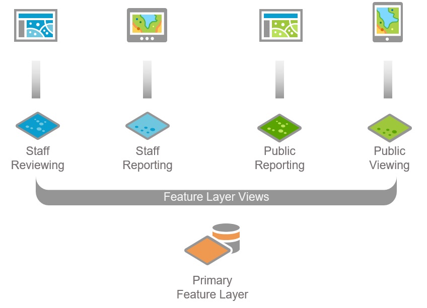
ESRI recently implemented new functionality into ArcGIS Online which greatly expands the ability of the webmaps that are created and hosted there. Called “Feature Layer Views”, this new type of data storage allows a commonly utilized symbolization method in desktop GIS to be applied to ArcGIS Online feature layers. In a desktop GIS application, a single spatial file can be represented in a dataframe one or more times. Each instance of the spatial file can have its own unique symbolization settings and templates applied to it. This is a great way to reduce duplication of efforts when creating maps , while at the same time visualizing information from more than one attribute.

Around the beginning of the new year, ESRI released new functionality to ArcGIS Online which facilitates this. As previously mentioned, this functionality is called “Feature Layer Views”, and a basic diagram of its usefulness can be seen below.

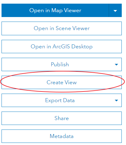
To begin creating and utilizing feature layer views, open up the feature layer which you would like to create a view for in the My Content section of ArcGIS Online by clicking on the layer name. You will notice to the right there are several options, select Create View.

Assign a unique title, description, tags, and a location to save the view and click OK. Open an existing webmap, or create a new webmap to display the data in. This can be different than the map in which data collection is being performed, or the same one. In many cases, it may be more desirable to create a new webmap strictly for displaying information and tracking the collection of data.

Once the webmap is open and the source feature layer and feature layer view have been added to the map, you can begin modifying symbology for one or both layers. Since, in the example I have been using, symbology was defined before uploading the feature layer, I will only demonstrate modifying the view’s symbology.

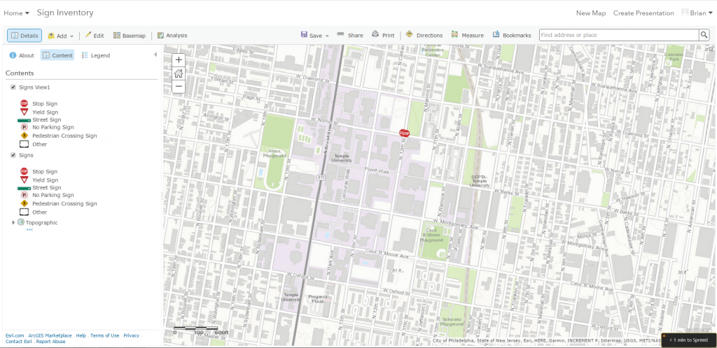
Feature Layer & Feature Layer View in the same webmap

Note the two layers listed in the image above. If data is added or modified to one of the layers, the change is reflected in both. Both the view and the source feature layer can be configured to allow or disallow editing and creation of data. In cases where a source layer and a view are in the same map, you may want to disable editing and creation of data in the view. However, if you want to utilize different symbolization throughout several different webmaps, you may want to allow editing and creation of data across both the feature layer and its view.

To change the attribute that a feature layer or view is being symbolized on, click on a feature layer or view’s name and then click “Change Style” (the button that appears as three shapes). Next, choose the new attribute you wish to symbolize on. A common use of views is to symbolize an attribute that represents a feature’s condition or status. This way, you can see the type of feature and an additional descriptive which may influence the action that needs to be taken on that feature.

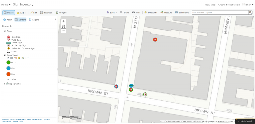
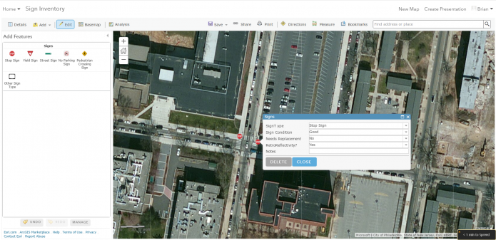
In the example I have been working with, which can be seen below, by adding a simple shape and associating a color to the condition attribute, we are able to see both the Signs Type and Condition without switching symbolization methods.

Signs Symbolized by Type and Condition

Importing Individual CAD Layers into GIS using ArcPy

Complex CAD files often come into the GIS software with an overwhelming amount of layers.   This makes it very difficult to work with the data to identify useful layers and often drastically slows down your computer.  This post will walk through a way to convert only the necessary CAD layers into a geodatabase, instead of sifting through the unneeded layers, lines, and details in GIS.  The demo script walks through my process of importing the room polygons of Temple’s Alter Hall and converting them to a geodatabase to later join with our university room database.

Step 1:  #Import System Modules

import arcpy

Don’t forget to import ArcPy!


Step 2: #Establish Workspace Environment

arcpy.env.workspace = “C:/Users/tug28727.TU/Desktop/cad_dwgs/alter”

This line establishes your workspace.  Select the location where your CAD Drawings are.  For my script I used the folder location for Alter Hall.


Step 3: # Create a value table

vTab = arcpy.ValueTable()

A value table is necessary to hold input feature classes when you run a merge later in the script.


Step 4: # Create Geodatabase

arcpy.CreateFileGDB_management(“C:/Users/tug28727.TU/Desktop/cad_dwgs/alter”, “alter.gdb”)

A geodatabase needs to be create to store all of the features.


Step 5: #Identify CAD drawings and Create Features from CAD Layers

for fd in arcpy.ListDatasets(“*.dwg”):
     layername = fd + “_Layer”
     # Select only the Polygon features on the drawing layer rooms
     arcpy.MakeFeatureLayer_management(fd + “/Polygon”, layername, “\”Layer\” = ‘RM$'”)
     vTab.addRow(layername)

First, this cycles through all of the files in the workspace and identifies those files that end in .dwg- which are the CAD files.  Next, it creates and layer name.  After that, it creates features searching for whatever CAD details you want to add (here I am searching for Polygons on the RM$ layer).  Lastly, the features are populated on the value table created in step 3.


Step 6: #Merge into one Feature Class

arcpy.Merge_management(vTab, “C:/Users/tug28727.TU/Desktop/cad_dwgs/alter/alter.gdb/rooms”)

This tool merges all of the CAD features from Step 5 into one feature class in the geodatabase we created in Step 4.  If you wanted to merge the value table with other data you would add brackets and commas separating the data to merge where the vTab is located (ex. [vTab, “alter_rooms.shp”], “C:/fake_cad_folder/all_buildings”).


This script should successfully search through your workspace files to identify CAD drawings, and bring in the layers you want in a geodatabase.   Step 5 is where you are able to change which CAD layer you are looking for.   This script hopefully streamlines your process of import CAD files into GIS.  ArcGIS has plenty of resources on CAD and GIS integration located here.


Gathering Data in the Field with the Collector for ArcGIS App

When I first started working with GIS, I often wondered, where did all of this spatial data come from? As I progressed through my initial undergrad coursework and internship experiences, the answers quickly revealed themselves. Some of the data is created by someone sitting at a desk. Other data is automatically generated as a subset or byproduct of another dataset. A large amount of data, however, is collected on-site, by people in the field.

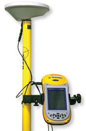
When I began my first internship I was doing exactly that. Weather permitting, I would be out in the field collecting data with a high-tech, high-end Trimble GPS.

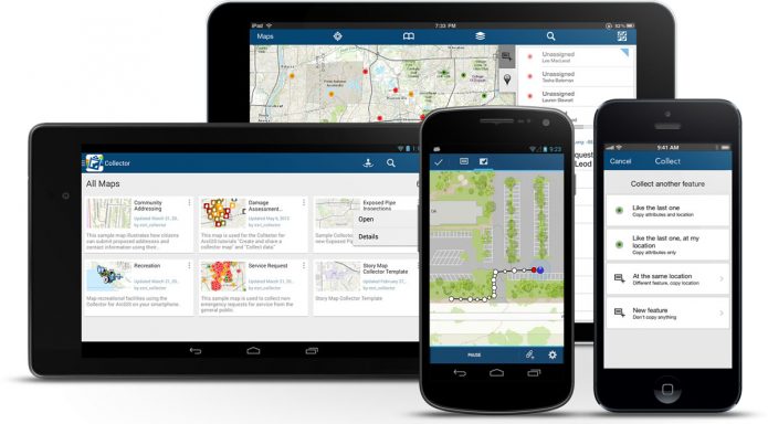
As many of us know, GIS does not typically have the capability or need to achieve survey-grade accuracy. For this reason, it has become an increasingly popular choice to skip purchasing a $10,000 GPS unit and instead purchase an Android tablet or iPad for $1000 or less. This trend has been on the rise ever since powerful tablets with an acceptable battery life for mobile data collection became an affordable option. Because of this, GIS software companies have developed native Android and iOS apps for mobile spatial data collection. There are several apps out there, including free and open source options. Data collection with these native apps can even be performed on a smart phone.

            Two Options for Mobile Data Collection

This post will focus on ESRI’s Collector for ArcGIS app, as it will tie in with the article I wrote two weeks ago detailing how to create and host a dataset in ArcGIS Online tailored for mobile data collection.

Collector for ArcGIS

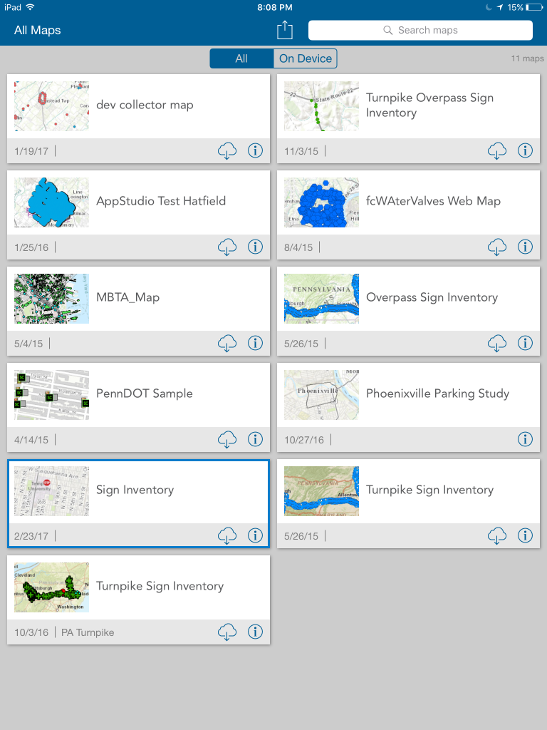
The Collector app is available on the Google Play store for Android and the App Store for iOS. After downloading the app, login to your organization’s account just as you would on ArcGIS Online. Any webmaps that exist in your organization’s ArcGIS Online account will be visible in the Collector’s main menu.

Collector for ArcGIS Main Menu

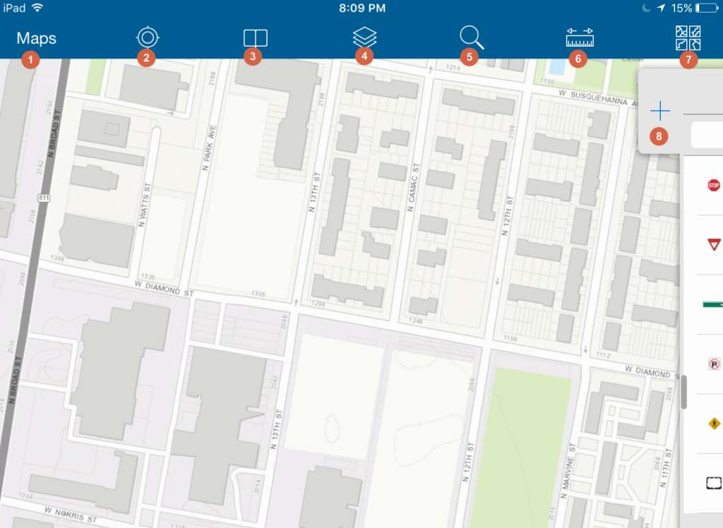
Select and open the map that you wish to collect data in. In this case, the Inventory map that was created in the previous blog post. The Collector’s map interface is relatively simple and its capabilities are intuitive and user friendly. Depending on your device, the layout may be slightly different, but the same functionality is present across all device types. Below is a screenshot of the initial Collector window, with a brief outline of what each button does.

  1.  The maps button will return to the main menu.
  2. The find my location button will use your device’s built in GPS to find your location and display it on the map.
  3. The bookmarks button allows for saving of specific locations / map extents as bookmarks. This eliminates the guesswork if you need to quickly reference or jump between two areas.
  4. If you are collecting more than one type of feature, the Layers tool is useful for turning on and off datasets when one type may not be in use.
  5. The search tool works like a Google Maps search, allowing you to search for and zoom to any location on Earth. It can also be configured to search through attribute values for a feature layer in the map.
  6. The measurement tool allows you to measure distances and areas by drawing temporary lines and polygons on the map.
  7. The basemap tool allows you to select and change the basemap. Available basemaps include Topographic, Imagery (and an option to include labels), OpenStreetMap, ESRI Streets, Terrain, and the USGS National Map, among others. You can also create and load a custom basemap if, for example, you have higher resolution imagery available for your study area.
  8. Clicking on or dragging the plus sign to the left will allow for the creation of new features. Feature templates defined in ArcMap or ArcGIS Online will be visible here for any feature layer that is present in the webmap.

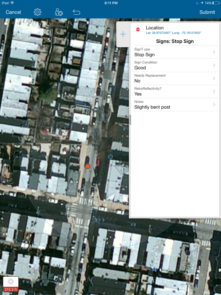
Once you’ve familiarized yourself with the tools available in the Collector, you can begin collecting data. Click on or pull the plus sign (point 8) to the left to see templates available for creation. On some versions of the Collector, the location of the feature will automatically be assigned your current location. If this doesn’t automatically begin, you can click the symbol that looks like a person with the find my location target next to it to use your location for the feature. You can also tap any location on the map to set the feature’s location to that point. The Collector also allows you to draw vertices for line and polygon feature layers this way. There is also the capability to “walk” a line or polygon feature, the Collector will drop a verticy at a predefined distance as you walk along a feature until you tell it to stop.

A Feature Collected in the Field

Next, you can begin assigning values to the attributes for that feature. Note that the domain value lists are present for the attributes that you configured to have them. This helps to greatly streamline a collection effort and can cut the time it takes to collect a single feature tremendously. Editing can be done in the field if any mistakes were made, and the progress of the inventory can be seen back at the office in real time as the collection effort occurs in the field.

In the next blog post, I will go further in how to utilize ArcGIS Online’s suite of tools to better represent, share, and understand the data that has been collected.

Georeferencing Floor Plans for Use in GIS

ArcGIS claims to have seamless integration between CAD and GIS.  However, this integration can be very confusing if your CAD floor plans are not georeferenced already.  Furthermore, the Georefencing toolbar in ArcGIS can be very time consuming to manually shift, rotate, and scale each floor plan one-by-one.   This post will look at an efficient way to georeference floor plans by building using the AutoCAD World File tool.

First, you would need to download the AutoCAD World File from this link.  This tool contains a .LSP script that will assign a world file to each .dwg file.  A world file contains the locations reference points in order for the GIS software to know where to place each floor plan when it is brought into the GIS software.


Step One: Export a shapefile to CAD

Right click on the shapefile of the buildings that contain the floor plans and select Data-> Export to CAD.  Next, export that shapefile in the DWG2013 format.  Leave the selection and seed file as they are.


Step Two: Open the shapefile CAD

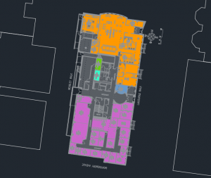
To do this, just open the .dwg file in the folder that it was saved in.  Once you open this file, you will notice it looks just like it would in GIS.  Furthermore, the coordinates are included at the bottom of the document showing that you are now working in a georeferenced plane.


Step Three:  Add the Floor Plan 

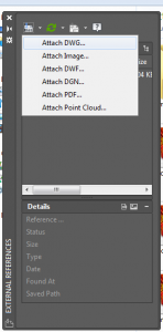
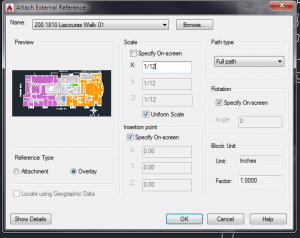
Type the command XREF in the bottom command bar and hit enter.  This will open a file reference box.  Open the drop-down menu under the DWG icon and select DWG.  Navigate to a floor plan you want to add and select it.  In the following window, under Scale de-select “Specify on Screen” and select Uniform Scale.  Enter 1/12 in the X box in order to convert feet to inches to scale the floor plans correctly.  Select “Specify On Screen” for Insertion Point and Rotation and leave Reference Type as “Overlay”.  Click OK.

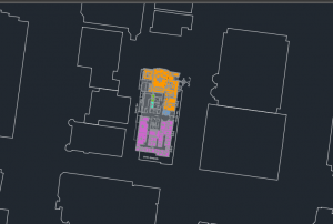
Select the point of insertion and rotation angle in order to place the floor plan.  Don’t worry if it isn’t exact because you can adjust it quite easily.


Step Four: Align Floor Plan

In order to adjust the floor plan so it aligns with the building footprint, type the command ALIGN in the command box.  Select your floor plan and hit enter.  Next, you will be instructed to select a minimum of two reference points.  Match up opposite corners of the floor plan to the building foot print.  I suggest you use more than two reference points to accomplish this.  You can do the ALIGN operation as many times as needed to get the floor plan precisely aligned to the footprint.


Step Five: Activate the AutoCAD World File App

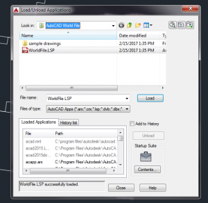
Type APPLOAD command into the command bar and locate the AutoCAD World File folder.  Select the WorldFile.LSP file and hit Load.  Wait for the box on the bottom to say “World File Loaded Successfully” and then hit close.


Step Six: Using the Tool to Create a World File

Type CREATEWORLDFILE command in the command bar and hit enter.  Select the floor plan (not the footprint!).  A Save File box will open with a file name esri_cad.wld.  Locate the folder that contains all the buildings floor plans and hit save.  Do not change the name of the .wld file.


Step Seven: Open the CAD Drawing in ArcGIS

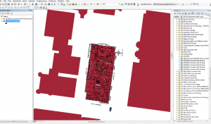
Open the same shapefile you used in this demo in ArcGIS.  Use the Catalog to navigate to where the building floor plans you just created a world file for is located.  Drag the floor plan file into the GIS window.  Now, the floor plan should drop right on top of the building footprint.


Notes:

This demo should work for all floor plans for the building.  However, in many buildings floors are not always the same size so the georeferencing may need to be tweaked to fit the footprint accurately.  Use the Georeferencing toolbar in ArcGIS to fix this.

CAD files can be pretty messy to work with in GIS, so I suggest only turning on the layers you actually need.  This can be accomplished by right clicking on each layer in the group and selecting Properties.  Next, select the drawing layers tab to turn off the layers you do not need to make the file easier to use. You can then convert this to a Layer or Feature Dataset or export it as a shapefile to make it even easier to use.

A youtube tutorial on using the AutoCAD World File tool is here.

Creating and Storing Your Data in the Cloud with ArcGIS Online

This post and several posts to follow will detail how to design, host, and implement an effective asset inventory using the ArcGIS for Desktop Suite and ArcGIS Online, in conjunction with the Collector for ArcGIS app (Android, iOS, Windows 10).

Note: In order to utilize the Collector for ArcGIS and publishing ArcGIS Online services from ArcMap, an ArcGIS Online subscription is required. 

Step 1: Creating a Dataset

If you are both designing and utilizing the dataset that will be created through the data collection effort, congratulations, you might already know exactly what you want to collect and how to design your feature classes and attributes. However, if you are developing a GIS solution for someone else, it is important to work closely with that person to identify exactly what information is going to be collected before there are people in the field collecting. It is much easier to make a change to a domain value / max field length before an ArcGIS feature layer is deployed to the cloud.

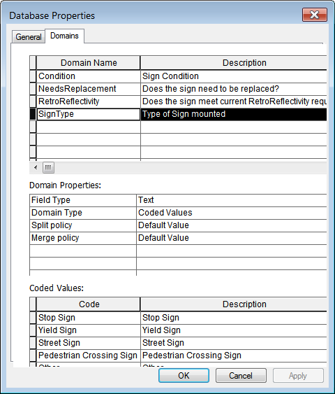
Fortunately, feature classes have built in quality assurance capabilities and they translate well into ArcGIS Online. These QA measures come in the form of domains. Domains in the ArcGIS for Desktop environment turn standard text attributes into dropdown lists. This is great for preventing varied user data entries (think Yield vs Yield Sign vs Yld).

Domain Definitions

Domain Definitions in an ArcGIS File Geodatabase


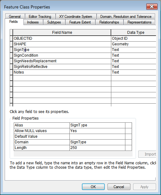
Feature Class Attribute Creation, with Domains Assigned

After that, create the feature class that will act as a template for the ArcGIS Online feature layer. Be sure to assign the domains to the appropriate attribute as you are creating attribution for the feature class. You can also define feature templates and symbology now, or after the feature layer is published to ArcGIS Online.

Step 2: Publishing Feature Classes to the Cloud

Add that newly created feature layer into an ArcMap session. As stated above, you can define templates and symbology now or later in the cloud. I opted for the former, because I liked the symbology options that were available in ArcMap.

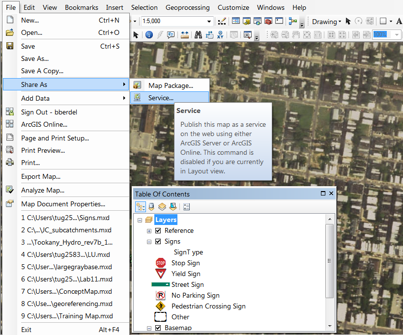
Publishing a Feature Class with Symbology Loaded into ArcMap

Sign in to your ArcGIS Online account via the File menu, and publish the service using File:Share As:Service (seen above). In the dialog window that appears, select Publish a Service and click next. Name the service, and click continue.

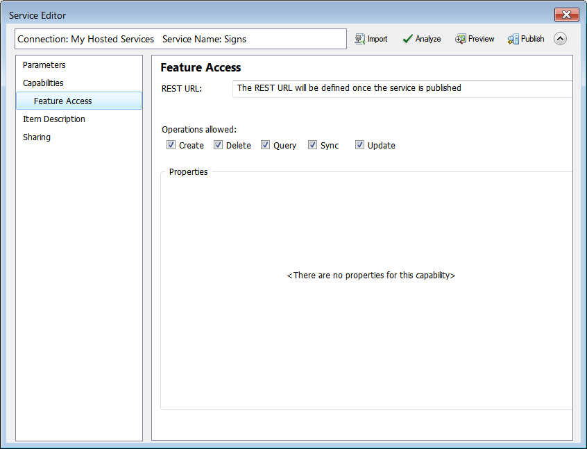
In the service editor that appears next, be sure that the service being published has the Feature Access option checked under Capabilities, as well as at least the Create and Update Operations allowed (seen below). Enter a summary and tags as required, and click the publish button to begin creating an ArcGIS Online Feature Layer.

Configuring a Feature Service to have Add and Edit Capabilities.

Step 3: ArcGIS Online & Beyond

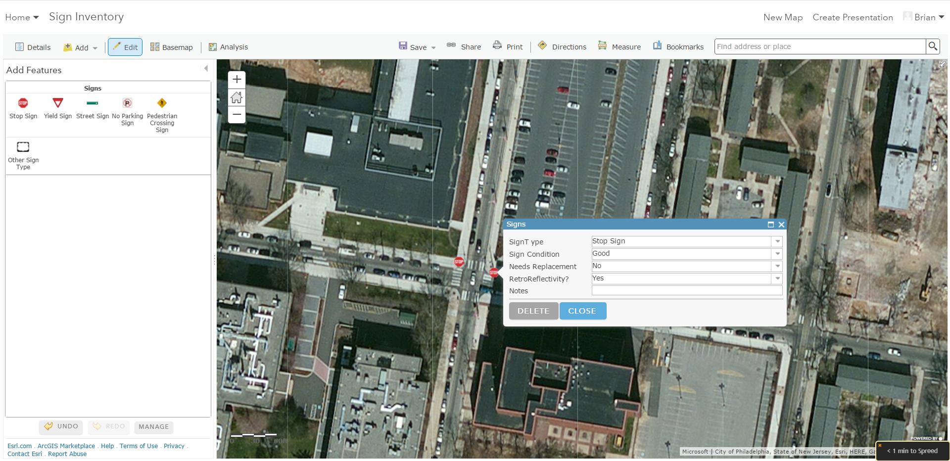
Log in to your ArcGIS Online account from your web browser. From your organization’s home page, click on My Content, this is where your newly published feature layer is being stored. Use the Create: Map menu item to create a new web map to utilize and share the feature layer. The new map will automatically open. Using the Add menu item, search for your newly created feature layer and add it to the map. Be sure to save the map after adding the feature layer.

From here, you can add data and alter symbology and the basemap. The webmap can be public facing or private, and shared via link or embedded into another website via HTML.

An ArcGIS Online Webmap with Fields and Domains Created in ArcGIS Desktop

In the next blog post, I will go into detail about collecting data with the Collector for ArcGIS app for mobile devices.