First Look at the New Indoor CAD to GIS Tool

To continue my series discussing CAD to GIS integration, I will look at ESRI’s new Indoor CAD to GIS Tool.  This tool is included with the newest update to ArcGIS Desktop 10.5 or ArcGIS Pro 10.4 and requires Microsoft Excel or LibreOffice/OpenOffice.  The tool was designed to conform to the American Institute of Architects (AIA) specifications for indoor spaces and is part of ESRI’s new collection of CampusViewerTools.

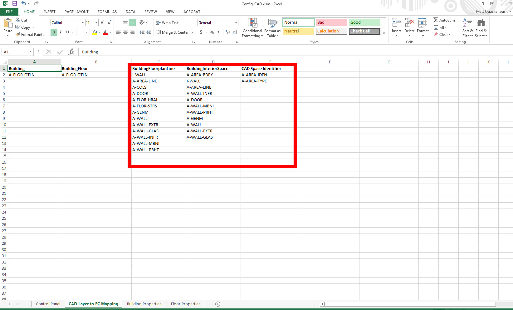
Where you need to specify which CAD layer is floor plan line, interior space, or identifier.

The tool uses an .xlsx worksheet with three tabs for the CAD Data.  The CAD LAYER TO FC MAPPING tab is where you manually separate all CAD layers as either Floor Plan Lines, Interior Spaces, or Identifiers.  The Building Properties Tab is where general building information such as Building Name or Date Built is stored to be included with all data imported.  The Floor Properties tab is where you identify the floors of the CAD layer and set the order, elevation, and ceiling heights for each floor- which is necessary if you plan on incorporating these into a 3D GIS.

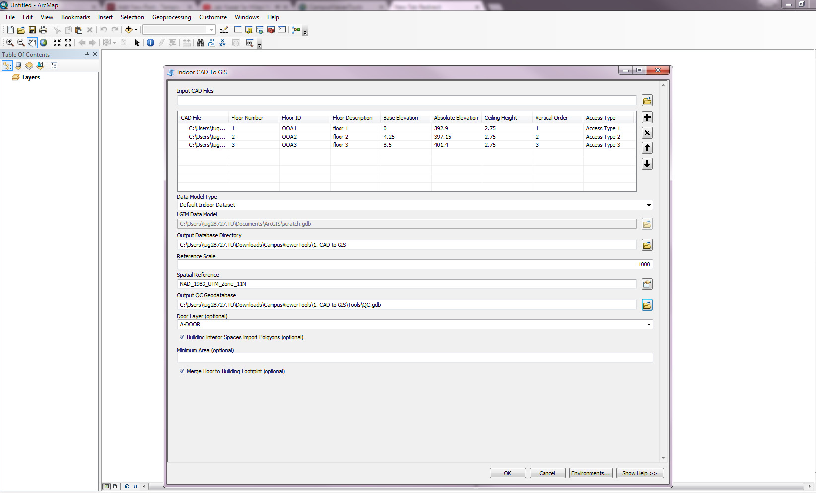
Running the tool in ArcGIS- very simple to use and most of the fields auto-populate when you open it.

Once the .xlsx worksheet is complete, you save it as a .csv so can be used in ArcGIS. Once in ArcGIS, you open navigate to the tool using your Catalog and much of the import is already auto-populated.  Just locate your .gdb to save it to and the spatial reference and run the tool.  When it’s done, you’ll see the gdb now has your building footprint, floor footprint, floor plan lines, and interior spaces ready to use.

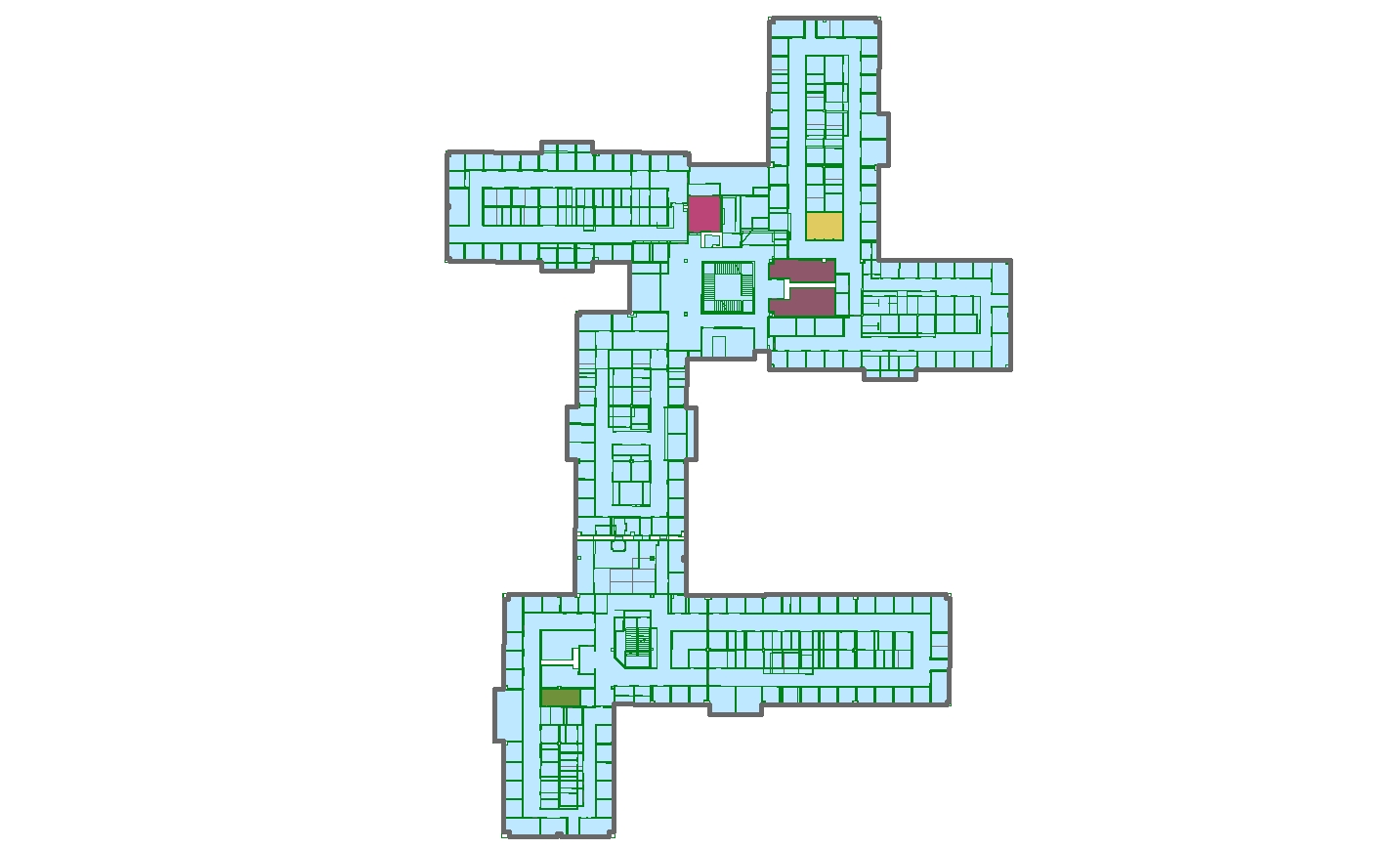
The resulting floor plan- looks great!

Ultimately, the new Indoor CAD to GIS Tool is very easy use and has great results.  As I’ve discussed in several posts, CAD to GIS conversion can be very messy and time-consuming, and the new Indoor CAD to GIS Tool is now an essential tool when doing this work.

It does have several limitations, being it requires your CAD data to have consistent layer naming and be in a real-world coordinate system.  If you are working with an entire campus of data that has a variety of layer naming standards and no coordinate system, it will take you several steps to even begin using this tool.  However, assigning a coordinate system and renaming layers within a consistent standard between drawings can both be accomplished using a Python script or a LISP script in AutoCAD.

The tool runs pretty slow (one building with 3 floors took just under 10 minutes) and any typo at any point in the spreadsheet can lead to the tool not working.  While it takes a while to populate the spreadsheets, it is still much quicker than manually importing the CAD files and cleaning them up one-by-one.

More info on the new Indoor CAD to GIS tool can be found HERE.

Land Classification and Land Use

After the completion of my Geo-referencing tasks (years 1995, 1975, and 1959), I was given the option between more Geo-referencing (1965) or a slightly different route, which consisted of creating a method to classify land types and land uses. If it wasn’t obvious by the title, I chose Geo-referencing 1965…

Land classification is the method of determining what a feature is on imagery purely based on pixel value (pixel value can be interpreted differently depending on the situation). This allows for a colorful rendition and separation, which results in an easy to read and visualize context of where different features are located. Results can vary and are heavily reliant on image quality. The lower quality the image or imagery, the more generalization and inaccuracy of the classifications.

Anyway, land classification can be simple and it can also be quite difficult. If you are using tools that already exist, or software that are built to classify imagery, you can easily begin land classification/land use. If you are using preexisting material it will quickly become a matter of finding the right combination of numbers in order to get the classifications you want. This method is not too difficult, just more tedious in regards to acquiring your result. However, if you approach it from scratch, it will be significantly more engaging. In order to approach it from the bottom up, you have to essentially dissect the process. You have to analyze your imagery, extract pixel values, group the pixel values, combine all of them into a single file, and finally symbolize them based on attribution or pixel value which was recorded earlier. It is much easier said than done.

I am currently approaching the task via already created tools, however if I had a choice in the matter, I would have approached it via the bottom up method and attempted to create it from scratch as there is more learning in that and it is much more appealing to me. Regardless, I am creating info files, or files that contain the numbers, ranges, and classifications I am using to determine good land classifications. In contrast to what I stated earlier, this is quite difficult for me as the imagery is low quality and I am not a fan of continuously typing in ranges until I thread the needle.

The current tool I am using is the reclassify tool that is available through the ESRI suite and it requires the Spatial Analyst extension. This tool allows for the input of a single image, ranges you would like to use to classify the selected image, and output file. After much testing, I am pretty sure there can only be a maximum of 24 classifications (which is probably more than enough). In addition, the tool can be batch ran (as most ESRI tools can be), which means it can be run on multiple images at once. This is a much needed features for many situations, as I presume most times, individuals are not going to classify one image and be done (or at least I am not going to be one and done).

That is an image that was reclassified using the reclassify tool. I am not sure how good of a classification this is as I have not fully grasped the tool yet and every time I give it ranges, it spits out the same generic ranges that I did not input (which is a bit frustrating, but it comes with the territory). I am sure it is human error though and not the tool messing up. I am not sure what the final result is supposed to be, but I will be sure to fill you in once I achieve it (if I ever do…).

Creating a Network Analysis Dataset and Generating a Service Area Layer

Network analysis can be an extremely beneficial tool for any organization which relies on GIS to understand the area it serves. This is particularly true if the organization deals primarily with transportation or the distribution of goods. The network analysis package through ArcGIS allows organizations to gain critical insight into how people and goods move around within their designated service or study area. More specifically, the engineers that I work with at McMahon utilize GIS network analysis to gain enhanced insight on the regions in which they serve as transportation engineers and planners. The baseline method of analysis utilized is creating a service area layer, or series of layers, to gain an understanding of how much distance can be traveled on a road network given a set of parameters.

A Basic Example of a Service Area Layer, With Three Interval Breaks

The first step in creating a service area layer is to create a network dataset. A network dataset is a special type of ESRI dataset, which contains both spatial layers and network layers, as well as custom preferences and parameters to fine tune the output of the network dataset. To create a network dataset, first, download a road network layer that represents the area in which you want to create service areas. Often times, these layers are available from government agencies. For example, all Pennsylvania state and local roads are available on PASDA, provided by PennDOT. Once the streets / roads layer is downloaded, it is important to clip the layer to what you expect you might utilize from the service area analysis. If you choose not to clip the layer, you may find creating and working with the network dataset to be slow and difficult to manage.

You will also need to create a source point file that will represent the location or locations from which the service areas will be generated. You can create the actual points either now or after the network dataset is created, but the point feature class itself needs to be created beforehand. You will also need to create a file geodatabase and feature dataset to store all of these layers and datasets in.

Once the layer is downloaded, clipped, and present in your working directory with the source point file you can create the network dataset. This can be done by right-clicking inside any feature dataset and clicking new > network dataset. A dialog window should appear with options regarding the new network dataset. Name the network dataset and click next. You can leave most of the settings at their default values unless otherwise instructed or if you know the network dataset will be used for purposes in addition to creating a service area. Finally, on the second to last page of options, check the box next to “build service area indexes”. This will speed up the creation of service areas in the future.

Creating a New Network Dataset Inside of a Feature Dataset

Click finish, and you will be asked if you want to build the network dataset. Click Yes. Once the network dataset has been created, open ArcMap and bring the newly created network dataset into the dataframe. When prompted to bring in any associated layers, say yes. Add the Network Analyst toolbar and click “New Service Area” under the Network Analyst dropdown.

Creating a New Service Area with Network Analyst

Click the button directly to the right of the Network Analyst dropdown, to open Network Analyst Window. Here, you can load any origin points (previously created), polygon or line barriers, as well as set options for the service area that is going to be created. You can drag the point layer which contains the origin points into the Facilities group. Clicking the Service Area Properties button (top right corner of the Network Analyst Window) will allow you to set important preferences for the service area that is about to be created. Some of the most useful settings include the accumulation tab, which allows you to track distance and time along the service area, and the analysis settings tab. The analysis settings tab will allow you to set the direction of the service area, as well as any breaks, and to implement a temporal aspect to the service area.

Service Area Properties

Apply any preferences and settings that have changed, and close the service area properties window. When everything is configured as desired, click the Solve button on the network analyst toolbar to run the analysis and create the service area. The analysis can be re-run an infinite number of times, and with the service area index that was created earlier, creating a service area should not take long each time. This way, you can tweak and fine tune the service area quickly and easily until you gain the desired result.

A Service Area Created Using Network Analyst