Map Link

Legendary folklorist Alan Lomax is celebrated for both the size and variety of his astounding collection. An esteemed ethnomusicologist, Lomax has cataloged the sounds of nearly 1,000 cultural groups from around the world, often giving voice to the poor or marginalized that wouldn’t be included on any record or in any museum. 

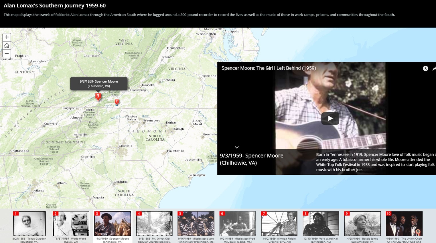
Lomax amassed a great deal of his most famous material during two trips to the American South in 1959 and 1960. During these trips, Lomax and his companion Shirley Collins wandered from Virginia to Mississippi with windows open listening for the voices of singers and musicians to interview, record, and photograph. Unbelievably, these trips resulted in the first stereo field recordings made in the South.

This story map offers a geographic visualization of these seminal trips for Southern American music. The map data was collected directly from the Lomax Family Collections at the American Folklife Center, part at the Library of Congress. This collection consists of more than 100 individual collections and includes 700 linear feet of manuscripts, 10,000 sound recordings,6,000 graphic images, and 6,000 moving images. Astoundingly, none of the material in the entire Lomax Collection contains any maps. Furthermore, the book “The Southern Journey of Alan Lomax: Word, Photographs, and Music” was used for supplemental information, as it offers more of a narrative story ­based structure than the abundance of documents in the Lomax Archive. 

The ten musicians for the map were selected because of their popularity in American Southern music as well as their variety of geography and musical genre.​These musicians were also included in the first CD that Lomax put out of his recordings from these trips, which were used for the music on the story map as well.

This story map successfully synthesizes multiple forms of media to show the viewer when, where, and who Alan recorded all during his iconic Southern Journey. Furthermore, the story map offers some unique insights into the spatial relationship between places on Lomax’s journey. For example, as you move out west there is a noticeable change in the tempo and style of the music. The music of Fred McDowell, Vera Ward Hall, and the prisoners at the Mississippi State Penitentiary in the Western portion of the map sounds much slower and drawn out than the more energetic sounds of Eastern musicians Bessie Jones, Wade Ward, and the Union Choir of the Church of God and Saints of Christ.

This map also successfully conceptualizes the nonlinear, meandering nature of the journey and helps pinpoint locations such as Northwestern Mississippi, Western Virginia, and around Norfolk, Virginia, where Lomax unearthed a hotbed of talented musicians that are now among the most important in American Southern music.

To continue my series discussing CAD to GIS integration, I will look at ESRI’s new Indoor CAD to GIS Tool.  This tool is included with the newest update to ArcGIS Desktop 10.5 or ArcGIS Pro 10.4 and requires Microsoft Excel or LibreOffice/OpenOffice.  The tool was designed to conform to the American Institute of Architects (AIA) specifications for indoor spaces and is part of ESRI’s new collection of CampusViewerTools.

Where you need to specify which CAD layer is floor plan line, interior space, or identifier.

The tool uses an .xlsx worksheet with three tabs for the CAD Data.  The CAD LAYER TO FC MAPPING tab is where you manually separate all CAD layers as either Floor Plan Lines, Interior Spaces, or Identifiers.  The Building Properties Tab is where general building information such as Building Name or Date Built is stored to be included with all data imported.  The Floor Properties tab is where you identify the floors of the CAD layer and set the order, elevation, and ceiling heights for each floor- which is necessary if you plan on incorporating these into a 3D GIS.

Running the tool in ArcGIS- very simple to use and most of the fields auto-populate when you open it.

Once the .xlsx worksheet is complete, you save it as a .csv so can be used in ArcGIS. Once in ArcGIS, you open navigate to the tool using your Catalog and much of the import is already auto-populated.  Just locate your .gdb to save it to and the spatial reference and run the tool.  When it’s done, you’ll see the gdb now has your building footprint, floor footprint, floor plan lines, and interior spaces ready to use.

The resulting floor plan- looks great!

Ultimately, the new Indoor CAD to GIS Tool is very easy use and has great results.  As I’ve discussed in several posts, CAD to GIS conversion can be very messy and time-consuming, and the new Indoor CAD to GIS Tool is now an essential tool when doing this work.

It does have several limitations, being it requires your CAD data to have consistent layer naming and be in a real-world coordinate system.  If you are working with an entire campus of data that has a variety of layer naming standards and no coordinate system, it will take you several steps to even begin using this tool.  However, assigning a coordinate system and renaming layers within a consistent standard between drawings can both be accomplished using a Python script or a LISP script in AutoCAD.

The tool runs pretty slow (one building with 3 floors took just under 10 minutes) and any typo at any point in the spreadsheet can lead to the tool not working.  While it takes a while to populate the spreadsheets, it is still much quicker than manually importing the CAD files and cleaning them up one-by-one.

More info on the new Indoor CAD to GIS tool can be found HERE.

Many of my posts this semester have discussed the integration of CAD and GIS for Temple’s campus to build a better campus map.  This is a process that many universities have been doing in order to understand more about the data that lives on their campus.  Having a better visualization of the campus ultimately improves the experience for students, staff, visitors, and the larger community.    Here are a few examples of institutions with excellent campus maps and what makes them impressive:

University of Arizona

The University of Arizona has an exceptional collection of campus data available on their website.  I picked University of Arizona for this list because they made several types of maps for different audiences- such as the public campus map, the private university interior map, or the campus sustainability map.  All the maps look different and are for unique audiences, yet still have a tremendous wealth of information, an easy to use interface, and look graphically appealing.

University of Maryland

A campus plant inventory!  Designated smoking areas! Bottle filling stations!  The University of Maryland campus map truly sets the bar for campus information.  Also, the map includes a helpful Overview Map and a search feature that is very easy to use.

Arizona State University

Arizona State has one of the most beautiful campus maps you will see.  They worked with the company CampusBird to produce a series of illustrative maps that look more like a classic retro video game instead of an education institution.  Additionally, they have a remarkable amount of information including the species of every tree on campus and high-quality panoramic images of campus landmarks.

ESRI Campus Viewer

The ESRI Campus Viewer is a demo campus application that ESRI is developing to make 3D campuses.  As you could see, it isn’t perfect but almost all applications visualizing floorplans in 3D struggle to be easy to navigate.  There is a fantastic wayfinding tool built in to get from room to room, but it still looks like there is some way to go until this is a viable option.  However, it’s worth keeping an eye on how the Campus Viewer tool is developed because it won’t be too long until universities start considering developing 3D campus maps.

Having a multitude of data on the campus means that different departments can work together to analyze campus problems.  For example, Campus Safety and Sustainability could work together to understand the patterns of bike thefts on campus.  Furthermore, emergency management can work with scheduling to understand when and where students are at certain times of the day in order to plan for an emergency.  This type of deeper understanding of the campus is essential to understanding how space is used on campus.

Complex CAD files often come into the GIS software with an overwhelming amount of layers.   This makes it very difficult to work with the data to identify useful layers and often drastically slows down your computer.  This post will walk through a way to convert only the necessary CAD layers into a geodatabase, instead of sifting through the unneeded layers, lines, and details in GIS.  The demo script walks through my process of importing the room polygons of Temple’s Alter Hall and converting them to a geodatabase to later join with our university room database.

Step 1:  #Import System Modules

import arcpy

Don’t forget to import ArcPy!

Step 2: #Establish Workspace Environment

arcpy.env.workspace = “C:/Users/tug28727.TU/Desktop/cad_dwgs/alter”

This line establishes your workspace.  Select the location where your CAD Drawings are.  For my script I used the folder location for Alter Hall.

Step 3: # Create a value table

vTab = arcpy.ValueTable()

A value table is necessary to hold input feature classes when you run a merge later in the script.

Step 4: # Create Geodatabase

arcpy.CreateFileGDB_management(“C:/Users/tug28727.TU/Desktop/cad_dwgs/alter”, “alter.gdb”)

A geodatabase needs to be create to store all of the features.

Step 5: #Identify CAD drawings and Create Features from CAD Layers

for fd in arcpy.ListDatasets(“*.dwg”):
     layername = fd + “_Layer”
     # Select only the Polygon features on the drawing layer rooms
     arcpy.MakeFeatureLayer_management(fd + “/Polygon”, layername, “\”Layer\” = ‘RM$'”)
     vTab.addRow(layername)

First, this cycles through all of the files in the workspace and identifies those files that end in .dwg- which are the CAD files.  Next, it creates and layer name.  After that, it creates features searching for whatever CAD details you want to add (here I am searching for Polygons on the RM$ layer).  Lastly, the features are populated on the value table created in step 3.

Step 6: #Merge into one Feature Class

arcpy.Merge_management(vTab, “C:/Users/tug28727.TU/Desktop/cad_dwgs/alter/alter.gdb/rooms”)

This tool merges all of the CAD features from Step 5 into one feature class in the geodatabase we created in Step 4.  If you wanted to merge the value table with other data you would add brackets and commas separating the data to merge where the vTab is located (ex. [vTab, “alter_rooms.shp”], “C:/fake_cad_folder/all_buildings”).

This script should successfully search through your workspace files to identify CAD drawings, and bring in the layers you want in a geodatabase.   Step 5 is where you are able to change which CAD layer you are looking for.   This script hopefully streamlines your process of import CAD files into GIS.  ArcGIS has plenty of resources on CAD and GIS integration located here.

ArcGIS claims to have seamless integration between CAD and GIS.  However, this integration can be very confusing if your CAD floor plans are not georeferenced already.  Furthermore, the Georefencing toolbar in ArcGIS can be very time consuming to manually shift, rotate, and scale each floor plan one-by-one.   This post will look at an efficient way to georeference floor plans by building using the AutoCAD World File tool.

First, you would need to download the AutoCAD World File from this link.  This tool contains a .LSP script that will assign a world file to each .dwg file.  A world file contains the locations reference points in order for the GIS software to know where to place each floor plan when it is brought into the GIS software.

Step One: Export a shapefile to CAD

Right click on the shapefile of the buildings that contain the floor plans and select Data-> Export to CAD.  Next, export that shapefile in the DWG2013 format.  Leave the selection and seed file as they are.

Step Two: Open the shapefile CAD

To do this, just open the .dwg file in the folder that it was saved in.  Once you open this file, you will notice it looks just like it would in GIS.  Furthermore, the coordinates are included at the bottom of the document showing that you are now working in a georeferenced plane.

Step Three:  Add the Floor Plan 

Type the command XREF in the bottom command bar and hit enter.  This will open a file reference box.  Open the drop-down menu under the DWG icon and select DWG.  Navigate to a floor plan you want to add and select it.  In the following window, under Scale de-select “Specify on Screen” and select Uniform Scale.  Enter 1/12 in the X box in order to convert feet to inches to scale the floor plans correctly.  Select “Specify On Screen” for Insertion Point and Rotation and leave Reference Type as “Overlay”.  Click OK.

Select the point of insertion and rotation angle in order to place the floor plan.  Don’t worry if it isn’t exact because you can adjust it quite easily.

Step Four: Align Floor Plan

In order to adjust the floor plan so it aligns with the building footprint, type the command ALIGN in the command box.  Select your floor plan and hit enter.  Next, you will be instructed to select a minimum of two reference points.  Match up opposite corners of the floor plan to the building foot print.  I suggest you use more than two reference points to accomplish this.  You can do the ALIGN operation as many times as needed to get the floor plan precisely aligned to the footprint.

Step Five: Activate the AutoCAD World File App

Type APPLOAD command into the command bar and locate the AutoCAD World File folder.  Select the WorldFile.LSP file and hit Load.  Wait for the box on the bottom to say “World File Loaded Successfully” and then hit close.

Step Six: Using the Tool to Create a World File

Type CREATEWORLDFILE command in the command bar and hit enter.  Select the floor plan (not the footprint!).  A Save File box will open with a file name esri_cad.wld.  Locate the folder that contains all the buildings floor plans and hit save.  Do not change the name of the .wld file.

Step Seven: Open the CAD Drawing in ArcGIS

Open the same shapefile you used in this demo in ArcGIS.  Use the Catalog to navigate to where the building floor plans you just created a world file for is located.  Drag the floor plan file into the GIS window.  Now, the floor plan should drop right on top of the building footprint.

Notes:

This demo should work for all floor plans for the building.  However, in many buildings floors are not always the same size so the georeferencing may need to be tweaked to fit the footprint accurately.  Use the Georeferencing toolbar in ArcGIS to fix this.

CAD files can be pretty messy to work with in GIS, so I suggest only turning on the layers you actually need.  This can be accomplished by right clicking on each layer in the group and selecting Properties.  Next, select the drawing layers tab to turn off the layers you do not need to make the file easier to use. You can then convert this to a Layer or Feature Dataset or export it as a shapefile to make it even easier to use.

A youtube tutorial on using the AutoCAD World File tool is here.