Land Classification and Land Use

After the completion of my Geo-referencing tasks (years 1995, 1975, and 1959), I was given the option between more Geo-referencing (1965) or a slightly different route, which consisted of creating a method to classify land types and land uses. If it wasn’t obvious by the title, I chose Geo-referencing 1965…

Land classification is the method of determining what a feature is on imagery purely based on pixel value (pixel value can be interpreted differently depending on the situation). This allows for a colorful rendition and separation, which results in an easy to read and visualize context of where different features are located. Results can vary and are heavily reliant on image quality. The lower quality the image or imagery, the more generalization and inaccuracy of the classifications.

Anyway, land classification can be simple and it can also be quite difficult. If you are using tools that already exist, or software that are built to classify imagery, you can easily begin land classification/land use. If you are using preexisting material it will quickly become a matter of finding the right combination of numbers in order to get the classifications you want. This method is not too difficult, just more tedious in regards to acquiring your result. However, if you approach it from scratch, it will be significantly more engaging. In order to approach it from the bottom up, you have to essentially dissect the process. You have to analyze your imagery, extract pixel values, group the pixel values, combine all of them into a single file, and finally symbolize them based on attribution or pixel value which was recorded earlier. It is much easier said than done.

I am currently approaching the task via already created tools, however if I had a choice in the matter, I would have approached it via the bottom up method and attempted to create it from scratch as there is more learning in that and it is much more appealing to me. Regardless, I am creating info files, or files that contain the numbers, ranges, and classifications I am using to determine good land classifications. In contrast to what I stated earlier, this is quite difficult for me as the imagery is low quality and I am not a fan of continuously typing in ranges until I thread the needle.

The current tool I am using is the reclassify tool that is available through the ESRI suite and it requires the Spatial Analyst extension. This tool allows for the input of a single image, ranges you would like to use to classify the selected image, and output file. After much testing, I am pretty sure there can only be a maximum of 24 classifications (which is probably more than enough). In addition, the tool can be batch ran (as most ESRI tools can be), which means it can be run on multiple images at once. This is a much needed features for many situations, as I presume most times, individuals are not going to classify one image and be done (or at least I am not going to be one and done).

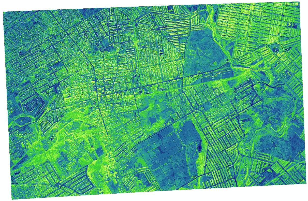
That is an image that was reclassified using the reclassify tool. I am not sure how good of a classification this is as I have not fully grasped the tool yet and every time I give it ranges, it spits out the same generic ranges that I did not input (which is a bit frustrating, but it comes with the territory). I am sure it is human error though and not the tool messing up. I am not sure what the final result is supposed to be, but I will be sure to fill you in once I achieve it (if I ever do…).

Geo-referencing: Understanding what you have time for and what you want, Quality VS. Time Spent

I have currently been Geo-referencing historic imagery for the past 3 months and would like to share my thoughts on some issues regarding project results and time.

As you may know, I am tasked with Geo-referencing historic imagery from the years 95′, 75′, and 59′ to the most recent imagery available to me, 2015. There are 140 images per year and about 105 of them that actually overlay the 2015 imagery. I have never done another Geo-referencing project of this size, so I am not sure if 105 images is a lot, but it seems like a lot. In addition, the images have to meet a certain accuracy standard, which is reasonable and understandable, while also tethering to each other on the edges. Essentially, images and imagery have to perfectly overlap and mosaic. These are all reasonable expectations from someone tasked with Geo-referencing.

However, time must be taken into consideration, especially during a task as tedious and vast as Geo-referencing. To give a little background, I began the tasks by originally putting in a conservative amount of control points (6-12) and lining up the images, however the edges would usually not line up due to camera positioning, sun angle, etc and this resulted in a revision, which is good for myself as I acquired more practice. During my revision, I focused on tethering the images together with a similar amount of control points (6-12), not so much lining them up to the imagery, although they did line up, just not as accurately or precisely as my first run through. This attempt also resulted in a revision, accompanied by a request to tether and accurately match the images to the imagery. This is where my post comes in.

In order to acquire both accurate and tethered imagery, I needed to place many more control points. Common sense would tell you that placing more data would require more time. Control points changed from 6-12 to 14-22, and placement and transformations became more prioritized. Image placement time skyrocketed from 5-10 minutes to 30 minutes – 1 hour. This quickly resulted in a scenario of something that could have been completed in a reasonable amount of time to something that may take months depending on your devotion to such a task.

The question for management becomes: Are we willing to spend such and such on a near perfect product or should we sacrifice some accuracy and quality for time and money. This question depends on what the Geo-referencing projects final use will be. In regards to my project, I am not sure the exact intent, but I think its eventual purpose will be public viewing. If that is the end goal, I think it would be best to skimp on some accuracy as the public does not generally have a professional eye and will not notice the small details such as perfect tethering and/or complete imagery line up.

Understanding Transformations within Geo-referencing: 1st Order and Spline

If you have ever been tasked with a Geo-referencing assignment, you may have heard of transformations. If you have not, or have never worked with Geo-referencing, transformations are essentially different algorithms that will determine how the image you’re Geo-referencing will shift, distort, bend, warp, or be altered. In regards to the ESRI suite’s (version 10.4) use of Geo-referencing, there are eight transformations (there may be more, but I have only been exposed to that offered by ESRI) available to you.

The transformations are as follows:

*In order to ‘unlock’ transformation for use, you need to meet a control point threshold

Zero polynomial – Essentially no image movement, just shifting

Similarity Polynomial – Image will move, but little to no distortion

1st Order Polynomial

2nd Order Polynomial*

3rd Order Polynomial*

Adjust – Significant emphasis on Control Points

Projective Transformation

Spline*


I tend to only use two transformations: 1st Order Polynomial and Spline. I am not an expert on Geo-referencing, so I tend to lean towards the ones I understand more easily. With that being said, those are the two I will discuss in further detail and how I have used them.

1st Order Polynomial:

This is a transformation that is available to the user the moment they start to Geo-reference an image. It requires no set amount of control points and allows for a consistent, but diminishing movement of the image you are working on. This consistency is what I like about this transformation and if you can successfully get an image to line up with your reference image in a few control points, this is the transformation for you.

However, the more control points you add, the less effective this transformation becomes. What I mean by that is within the first 6 control points, your image will shift greatly and begin to quickly line up with your reference, but after that threshold, the shifts become minimal and the amount of control points you have to add to gain the same effect rapidly get out of hand, which leads into the next transformation: Spline.

Spline:

Spline is a transformation that benefits heavily with the amount of control points you have. This transformation requires at least 10 control points be in play before you can even begin using it. It requires a lot of control points because it heavily distorts the images, essentially moving a part of your image exactly to the control point location. This is also a great detriment to the transformation. If you wish to use this transformation, you must place control points everywhere on your image, which can mean anywhere from 50-150+ control points, or else you are prone to having some parts of your image lining up and others being completely off.

Spline is very picky and requires delicate positioning of control points. Because they distort a given area, and you require a lot in order to maximize the effectiveness, you need to be careful with where you place them. If two or more control points are too close to each other, you will witness extreme warping in that location and will likely acquire the opposite effect of what you are looking for (unless you are an art major or artist, then you might find what you want).


To summarize both transformations within a sentence or two, 1st Order is a transformation if you want satisfactory, but not perfect Geo-referencing and you are on a time budget, while Spline is something you should use if you want a perfectly Geo-referenced image and have a lot more time available to you.

This should help transition into my next blog post: Understanding what you want and what you have time for within Geo-referencing.