As mentioned in an earlier post, I’m teaching a new general education class entitled “Evil Plots” about how graphs, maps and other forms of visual data communication can be used to persuade or mislead. The idea is to teach students to be informed consumer of data. My hope is that along the way they will learn foundations of proper data visualization and some tools they can apply in their own studies, whatever their major. Evil plots is not just about the graphical trickery. Sometimes the problem is not with the graph but with the data. Detecting fraudulent data is its own field, but surprisingly effective and easy to implement technique is to test whether the data comply with Benford’s Law.
In brief, Benford discovered that is you have data that spans many orders of magnitude — populations of cities in the U.S., the length of streams and rivers, even financial data — that it is six times more likely that the numbers will start with a 1 than a 9. In fact, the frequency distribution looks like this (from Wikipedia):

The this seems counterintuitive, but is actually a consequence of the numbers spanning such a wide range of values. The law fails for quantities that have a limited range, such as people’s height in meters, where I challenge you to find value starting with 9. There is a nice video introduction to Benford’s Law here, and here is a short video how Benford’s Law can be used to detect fraud. It seems that when people make up numbers to fudge their expense accounts or cook their books, few think to fabricate in accordance with Benford. One hopes I’m not simple educating my students to be better cheats!
Here is the simple case I had my students run by hand. The data are actually from a court case of fraudulent expenditures. Yes, Benford’s Law is permissible in court as evidence of fraud!
| Checks | First Digit | Count | |
| $1,927.48 | 1 | ||
| $27,902.31 | 2 | ||
| $86,241.90 | 3 | ||
| $72,117.46 | 4 | ||
| $81,321.75 | 5 | ||
| $97,473.96 | 6 | ||
| $93,249.11 | 7 | ||
| $89,658.16 | 8 | ||
| $87,776.89 | 9 | ||
| $92,105.83 | |||
| $79,949.16 | |||
| $87,602.93 | |||
| $96,879.27 | |||
| $91,806.47 | |||
| $84,991.67 | |||
| $90,831.83 | |||
| $93,766.67 | |||
| $88,336.72 | |||
| $94,639.49 | |||
| $83,709.26 | |||
| $96,412.21 | |||
| $88,432.86 | |||
| $71,552.16 |
Just count the frequencies of the numbers starting with, 1, 2, etc., then plot the distribution. Bam! Benford’s got you!
Benford and Geophysics
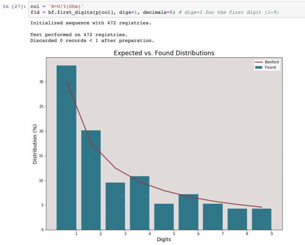
Out of curiosity, I decided to run Benford’s against some of my own geophysical data, specifically, apparent resistivity measurements from a sounding at a site on Temple’s Ambler Campus. The details aren’t important for Benford, but what is important is that apparent resistivity measurements typically follow a log-normal distribution with their being orders of magnitude between the mosts and least resistive parts of survey line. To do the calculation, I took advantage of a free package written in python (https://github.com/milcent/benford_py). Isn’t open source wonderful? The site also includes a photo of Benford and information on the history of his discover (and he wasn’t the first!) along with math details.
So I loaded my data into a Jupyter notebook and check it against Benford. Here is the result:
This is only a cursory exploration, but I encourage you to test you own data sets against Benford’s law. Send me an email if you discover something interesting!

