Measuring Similarity Between Texts in Python

By Luling Huang

This post demonstrates how to obtain an n by n matrix of pairwise semantic/cosine similarity among n text documents. Finding cosine similarity is a basic technique in text mining. My purpose of doing this is to operationalize “common ground” between actors in online political discussion (for more see Liang, 2014, p. 160).

The tools are Python libraries scikit-learn (version 0.18.1; Pedregosa et al., 2011) and nltk (version 3.2.2.; Bird, Klein, & Loper, 2009). Perone’s (2011a; 2011b; 2013) three-piece web tutorial is extremely helpful in explaining the concepts and mathematical logics. However, some of these contents have not kept up with scikit-learn’s recent update and text preprocessing was not included. This post addresses these issues.

If you are familiar with cosine similarity and more interested in the Python part, feel free to skip and scroll down to Section III.

I. What’s going on here?

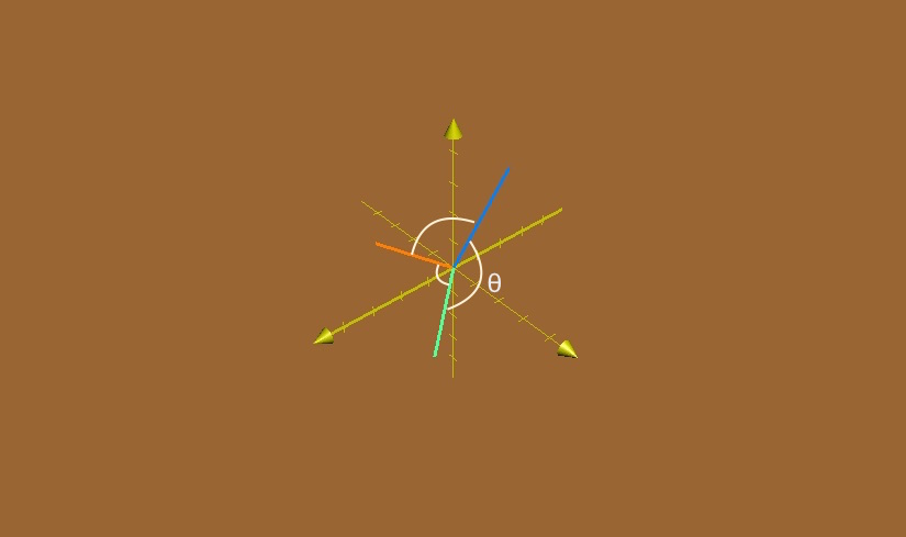
The cosine similarity is the cosine of the angle between two vectors. Figure 1 shows three 3-dimensional vectors and the angles between each pair. In text analysis, each vector can represent a document. The greater the value of θ, the less the value of cos θ, thus the less the similarity between two documents.

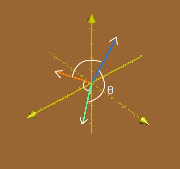
Figure 1. Three 3-dimensional vectors and the angles between each pair. Blue vector: (1, 2, 3); Green vector: (2, 2, 1); Orange vector: (2, 1, 2).

In math equation:

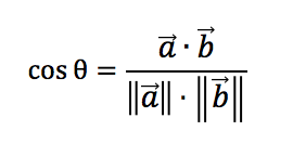
where cosine is the dot/scalar product of two vectors divided by the product of their Euclidean norms.

II. How to quantify texts in order to do the math?

a. Raw texts are preprocessed with the most common words and punctuation removed, tokenization, and stemming (or lemmatization).

b. A dictionary of unique terms found in the whole corpus is created. Texts are quantified first by calculating the term frequency (tf) for each document. The numbers are used to create a vector for each document where each component in the vector stands for the term frequency in that document. Let n be the number of documents and m be the number of unique terms. Then we have an n by m tf matrix.

c. The core of the rest is to obtain a “term frequency-inverse document frequency” (tf-idf) matrix. Inverse document frequency is an adjustment to term frequency. This adjustment deals with the problem that generally speaking certain terms do occur more than others. Thus, tf-idf scales up the importance of rarer terms and scales down the importance of more frequent terms relative to the whole corpus.

The idea of the weighting effect of tf-idf is better expressed in the two equations below (the formula for idf is the default one used by scikit-learn (Pedregosa et al., 2011): the 1 added to the denominator prevents division by 0, the 1 added to the nominator makes sure the value of the ratio is greater than or equal to 1, the third 1 added makes sure that idf is greater than 0, i.e., for an extremely common term t for which n = df(d,t), its idf is at least not 0 so that its tf still matters; Note that in Perone (2011b) there is only one 1 added to the denominator, which results in negative values after taking the logarithm for some cases. Negative value is difficult to interpret):

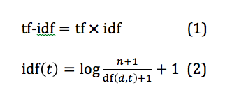
where n is the total number of documents and df(d, t) is the number of documents in which term t appears. In Equation 2, as df(d, t) gets smaller, idf(t) gets larger. In Equation 1, tf is a local parameter for individual documents, whereas idf is a global parameter taking the whole corpus into account.

Therefore, even the tf for one term is very high for document d1, if it appears frequently in other documents (with a smaller idf), its importance of “defining” d1 is scaled down. On the other hand, if a term has high tf in d1 and does not appear in other documents (with a greater idf), it becomes an important feature that distinguishes d1 from other documents.

d. The calculated tf-idf is normalized by the Euclidean norm so that each row vector has a length of 1. The normalized tf-idf matrix should be in the shape of n by m. A cosine similarity matrix (n by n) can be obtained by multiplying the if-idf matrix by its transpose (m by n).

III. Python it

A simple real-world data for this demonstration is obtained from the movie review corpus provided by nltk (Pang & Lee, 2004). The first two reviews from the positive set and the negative set are selected. Then the first sentence of these for reviews are selected. We can first define 4 documents in Python as: 

1
2
3
4
5

 d1 = "plot: two teen couples go to a church party, drink and then drive."
 d2 = "films adapted from comic books have had plenty of success , whether they're about superheroes ( batman , superman , spawn ) , or geared toward kids ( casper ) or the arthouse crowd ( ghost world ) , but there's never really been a comic book like from hell before . "
 d3 = "every now and then a movie comes along from a suspect studio , with every indication that it will be a stinker , and to everybody's surprise ( perhaps even the studio ) the film becomes a critical darling . "
 d4 = "damn that y2k bug . "
 documents = [d1, d2, d3, d4]

a. Preprocessing with nltk

The default functions of CountVectorizer and TfidfVectorizer in scikit-learn detect word boundary and remove punctuations automatically. However, if we want to do stemming or lemmatization, we need to customize certain parameters in CountVectorizer and TfidfVectorizer. Doing this overrides the default tokenization setting, which means that we have to customize tokenization, punctuation removal, and turning terms to lower case altogether.

Normalize by stemming:

1
2
3
4
5
6
7
8

 import nltk, string, numpy
 nltk.download('punkt') # first-time use only
 stemmer = nltk.stem.porter.PorterStemmer()
 def StemTokens(tokens):
     return [stemmer.stem(token) for token in tokens]
 remove_punct_dict = dict((ord(punct), None) for punct in string.punctuation)
 def StemNormalize(text):
     return StemTokens(nltk.word_tokenize(text.lower().translate(remove_punct_dict)))

Normalize by lemmatization:

1
2
3
4
5
6
7

 nltk.download('wordnet') # first-time use only
 lemmer = nltk.stem.WordNetLemmatizer()
 def LemTokens(tokens):
     return [lemmer.lemmatize(token) for token in tokens]
 remove_punct_dict = dict((ord(punct), None) for punct in string.punctuation)
 def LemNormalize(text):
     return LemTokens(nltk.word_tokenize(text.lower().translate(remove_punct_dict)))

If we want more meaningful terms in their dictionary forms, lemmatization is preferred.

b. Turn text into vectors of term frequency:

1
2
3

 from sklearn.feature_extraction.text import CountVectorizer
 LemVectorizer = CountVectorizer(tokenizer=LemNormalize, stop_words='english')
 LemVectorizer.fit_transform(documents)

Normalized (after lemmatization) text in the four documents are tokenized and each term is indexed:

print LemVectorizer.vocabulary_

Out:

{u'spawn': 29, u'crowd': 11, u'casper': 5, u'church': 6, u'hell': 20,
 u'comic': 8, u'superheroes': 33, u'superman': 34, u'plot': 27, u'movie': 24,
 u'book': 3, u'suspect': 36, u'film': 17, u'party': 25, u'darling': 13, u'really': 28, 
 u'teen': 37, u'everybodys': 16, u'damn': 12, u'batman': 2, u'couple': 9, u'drink': 14,
 u'like': 23, u'geared': 18, u'studio': 31, u'plenty': 26, u'surprise': 35, u'world': 39,
 u'come': 7, u'bug': 4, u'kid': 22, u'ghost': 19, u'arthouse': 1, u'y2k': 40,
 u'stinker': 30, u'success': 32, u'drive': 15, u'theyre': 38, u'indication': 21,
 u'critical': 10, u'adapted': 0}

And we have the tf matrix:

tf_matrix = LemVectorizer.transform(documents).toarray()
print tf_matrix

Out:

[[0 0 0 0 0 0 1 0 0 1 0 0 0 0 1 1 0 0 0 0 0 0 0 0 0 1 0 1 0 0 0 0 0 0 0 0 0
  1 0 0 0]
 [1 1 1 2 0 1 0 0 2 0 0 1 0 0 0 0 0 1 1 1 1 0 1 1 0 0 1 0 1 1 0 0 1 1 1 0 0
  0 1 1 0]
 [0 0 0 0 0 0 0 1 0 0 1 0 0 1 0 0 1 1 0 0 0 1 0 0 1 0 0 0 0 0 1 2 0 0 0 1 1
  0 0 0 0]
 [0 0 0 0 1 0 0 0 0 0 0 0 1 0 0 0 0 0 0 0 0 0 0 0 0 0 0 0 0 0 0 0 0 0 0 0 0
  0 0 0 1]]

This should be a 4 (# of documents) by 41 (# of terms in the corpus). Check its shape:

tf_matrix.shape

Out:

(4, 41)

c. Calculate idf and turn tf matrix to tf-idf matrix:

Get idf:

1
2
3
4

 from sklearn.feature_extraction.text import TfidfTransformer
 tfidfTran = TfidfTransformer(norm="l2")
 tfidfTran.fit(tf_matrix)
 print tfidfTran.idf_

Out:

1
2
3
4
5
6
7

[ 1.91629073  1.91629073  1.91629073  1.91629073  1.91629073  1.91629073
  1.91629073  1.91629073  1.91629073  1.91629073  1.91629073  1.91629073
  1.91629073  1.91629073  1.91629073  1.91629073  1.91629073  1.51082562
  1.91629073  1.91629073  1.91629073  1.91629073  1.91629073  1.91629073
  1.91629073  1.91629073  1.91629073  1.91629073  1.91629073  1.91629073
  1.91629073  1.91629073  1.91629073  1.91629073  1.91629073  1.91629073
  1.91629073  1.91629073  1.91629073  1.91629073  1.91629073]

Now we have a vector where each component is the idf for each term. In this case, the values are almost the same because other than one term, each term only appears in 1 document. The exception is the 18th term that appears in 2 document. We can corroborate the result.

import math
def idf(n,df):
    result = math.log((n+1.0)/(df+1.0)) + 1
    return result
print "The idf for terms that appear in one document: " + str(idf(4,1))
print "The idf for terms that appear in two documents: " + str(idf(4,2))

Out:

The idf for terms that appear in one document: 1.91629073187
The idf for terms that appear in two documents: 1.51082562377

which is exactly the same as the result from TfidfTransformer. Also, the idf is indeed smaller when df(d, t) is larger.

d. Get the tf-idf matrix (4 by 41):

tfidf_matrix = tfidfTran.transform(tf_matrix)
print tfidf_matrix.toarray()

Here what the transform method does is multiplying the tf matrix (4 by 41) by the diagonal idf matrix (41 by 41 with idf for each term on the main diagonal), and dividing the tf-idf by the Euclidean norm. This output takes too much space and you can check it by yourself.

e. Get the pairwise similarity matrix (n by n):

cos_similarity_matrix = (tfidf_matrix * tfidf_matrix.T).toarray()
print cos_similarity_matrix

Out:

array([[ 1.        ,  0.        ,  0.        ,  0.        ],
       [ 0.        ,  1.        ,  0.03264186,  0.        ],
       [ 0.        ,  0.03264186,  1.        ,  0.        ],
       [ 0.        ,  0.        ,  0.        ,  1.        ]])

The matrix obtained in the last step is multiplied by its transpose. The result is the similarity matrix, which indicates that d2 and d3 are more similar to each other than any other pair.

f. Use TfidfVectorizer instead:

Scikit-learn actually has another function TfidfVectorizer that combines the work of CountVectorizer and TfidfTransformer, which makes the process more efficient.

from sklearn.feature_extraction.text import TfidfVectorizer
TfidfVec = TfidfVectorizer(tokenizer=LemNormalize, stop_words='english')
def cos_similarity(textlist):
    tfidf = TfidfVec.fit_transform(textlist)
    return (tfidf * tfidf.T).toarray()
cos_similarity(documents)

Out:

array([[ 1.        ,  0.        ,  0.        ,  0.        ],
       [ 0.        ,  1.        ,  0.03264186,  0.        ],
       [ 0.        ,  0.03264186,  1.        ,  0.        ],
       [ 0.        ,  0.        ,  0.        ,  1.        ]])

which returns the same result.

References

Bird, S., Klein, E., & Loper, E. (2009). Natural language processing with Python: Analyzing text with the natural language toolkit. Sebastopol, CA: O’Reilly Media.

Liang, H. (2014). Coevolution of political discussion and common ground in web discussion forum. Social Science Computer Review, 32, 155-169. doi:10.1177/0894439313506844

Pang, B., & Lee, L. (2004). Sentiment polarity dataset version 2.0 [Data file]. Retrieved from http://www.nltk.org/nltk_data/

Pedregosa, F., Varoquaux, G., Gramfort, A., Michel, V., Thirion, B., Grisel, O., . . . Duchesnay, E. (2011). Scikit-learn: Machine learning in Python. Journal of Machine Learning Research, 12, 2825-2830. http://www.jmlr.org/papers/v12/pedregosa11a.html

Perone, C. S. (September 18, 2011a). Machine learning :: Text feature extraction (tf-idf) – Part I [Blog]. Retrieved from http://blog.christianperone.com/2011/09/machine-learning-text-feature-extraction-tf-idf-part-i/

Perone, C. S. (October 3, 2011b). Machine learning :: Text feature extraction (tf-idf) – Part II [Blog]. Retrieved from http://blog.christianperone.com/2011/10/machine-learning-text-feature-extraction-tf-idf-part-ii/

Perone, C. S. (September 12, 2013). Machine learning :: Cosine similarity for vector space models (Part III) [Blog]. Retrieved from http://blog.christianperone.com/2013/09/machine-learning-cosine-similarity-for-vector-space-models-part-iii/