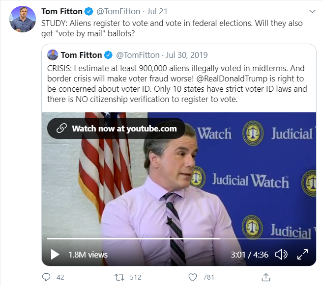
I saw this tweet by the president of the right-wing thinktank Judicial Watch and I was curious how he arrived at those numbers. In the video he cites a 2014 study by Jesse Richman and colleagues purporting to quantify the extent to which non-citizens voted in the United States, which is nearly illegal everywhere in the country (except some localities in Maryland). In this post I just want to address the Richman study (although I realize I am a latecomer to this study); how Fitton used its findings may be gristle for another post.
The Richman study
Richman et al. use the 2008 and 2010 waves of the Cooperative Congressional Election Study (CCES). This is an online survey done by YouGov and respondents are sampled from YouGov’s panels. Essentially, people volunteer to be on-going survey takers for YouGov and they provide demographic information to the company. So when a client approaches YouGov–say, the consortium of political scientists who want to study voters in congressional elections–they can tell YouGov that they want a cross-section of American adult citizens. In this case, the CCES team turned to existing data on U.S. citizens and figured out what a representative sample of U.S. voting-aged citizens would look like in terms of gender, age, race, region, education, interest in politics, marital status, party identity, ideology, religion, church attendance, income, voter registration status, and urbanicity. YouGov used this information to sample people from their panel to provide a “representative” sample of adult citizens. When the data are actually being analyzed, researchers can use weights to make sure that certain categories or combinations of individuals are not overrepresented.
As luck would have it, despite trying to get a representative sample of U.S. voting-aged citizens, the CCES scooped up a couple of hundred of non-citizens in both the 2008 and 2010 waves so Richman et al. studied them.
Besides using an online survey, the virtue of the 2008 CCES is that it used official records to verify respondents’ voter registration and voter participation.
Richman et al. find that around 15% of the noncitizens in the 2008 CCES and 2010 CCES say they are registered to vote. From the subsample of the 2008 CCES where the researchers were able to link respondents to official voting records, Richman et al. find that of the noncitizens who said they were registered, only 65% actually were registered, and of the noncitizens who said they were not registered, 18% actually were. So they infer that in both 2008 and 2010, 25% of non-citizens were registered to vote (15*.65 + 85*.18).
As an aside, the authors’ writing could have been clearer. They authors throw around different sample sizes (it was not clear to me what was the size of the sample linked to official records–94 or 140) and I could not figure out the actual tabulations they used to get the 65% and 18% figures. To be clear, I am not accusing them of finagling the analyses, just sloppy writing. They also wrote up these conditional percentages in a very confusing way :
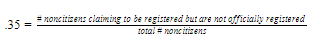
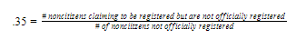
…our best guess at the true percentage of non-citizens registered…uses the 94 (weighted) non-citizens…match[ed] to commercial and/or voter databases to estimate the portion of non-citizens who either claim to be registered when they are not (35%) or claim not to be registered when they are (18%). [pp. 151-152]
It is not obvious what exactly the 35% and 18% figures are–that is, what exactly the denominator is. Taking the 35% figure for instance, is it this:
(no!)
or this?
(no!)
Or this?
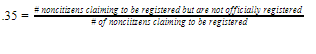
(yes!)
As far as voting goes, in 2008, 27 non-citizen respondents (8%) reported they voted, and in 2010, 13 (3%) reported they voted. Using similar math that I laid out above, Richman et al. estimate that in 2008, 6% of non-citizens voted, and in 2010, 2% voted. Richman look at the political preferences of these very small samples and concluded that non-citizen voters lean heavily Democratic. Based onthese nation-wide estimates of non-citizen voting and non-citizen voter political preferences and location-specific estimates of non-citizen residents, they conclude that non-citizen voters may have thrown elections in certain contests (namely, Obama’s victory in North Carolina in 2008 and Al Franken’s Senate victory in Minnesota in 2008).
Richman et al. find that unlike for the general population, the highly-educated are not more likely to vote. Indeed, among non-citizens, the association is negative, from which they conclude that non-citizen voting is mostly accidental and done out of ignorance that it is illegal.
The Richman Study — what can we say about noncitizen voting?
It is tempting to dismiss the CCES data on the grounds that while the respondents may be demographically representative of the broader population, some unmeasured characteristics might set them apart from other people. For instance, people who like taking surveys and join online survey panels just might be …weird. In reality, the best online polls have a track record that is comparable to more traditional phone polling. The Pew Research Center has shown this is the case specifically for looking at voter registration, and the documentation for the 2008 CCES provides evidence of YouGov’s impressive track record for previous surveys–in particular, I am struck by the 2006 CCES’s lack of bias in predicting state-wide elections. So just because it is online does not mean we can just throw out the data.
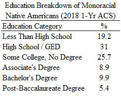
Having said that, I think there are real questions to be asked about how representative the sample of noncitizens are in the CCES, especially since the CCES team asked YouGov to draw a sample representative of adult U.S. citizens. Indeed, according to Richman et al., only 1% of the 2008 and 2010 CCES respondents reported being non-citizens. In reality, Census data indicate that in the late 2000s, non-citizens made up 8 percent of voting-age adults in the United States.
Richman et al. acknowledge this issue, somewhat. They note (p. 151) that their sample of non-citizen adults is much better educated than the population of non-citizen adults, and their fix for this issue to use sample weights (essentially weigh the highly-educated non-citizens less and weigh the less-educated non-citizens more). But this assumes that selection into the CCES is driven only by the observed factors that are the basis of the weights, like education. So if you correct for the education imbalance, then you can generalize to the rest of non-citizen voting-aged adults, right?
That seems to me an awfully heroic assumption. I would guess that the non-citizens who select into the CCES study are an unusual group, composed of people interested in domestic politics but are either (a) unaware that political researchers are not interested in them because they can’t vote or (b) unaware they should not be voting. My hunch is that the CCES sample is reflecting a small segment of the non-citizen population predisposed to vote. I find it very unlikely that 25% of non-citizens were registered to vote in the late 2000s, or that 6% voted in the 2008 presidential election. In other words, my hunch is that Richman et al. are using a biased sample. When I say biased, I mean, in the sense that if you replicated the sampling methodology over and over, you would consistently over-estimate non-citizen voter registration and voter participation.
Richman et al. argue that the bias could go the other way–that non-citizens voters savvy enough to know they are committing a crime are going to be underrepresented in the data. But how common is such a person? Social scientists have talked about how voting is irrational even for citizens. How much more irrational would it be to vote if it means committing crime and/or being deported from a country one presumably wants to stay in?
I am also really, really, not crazy about generalizing from the really small samples of self-confessed non-citizen voters to (a) non-citizens as a whole, and (b) applying those generalizations to non-citizen voters in particular contests, which just assumes that the distribution of political views among non-citizens is invariant across different contexts.
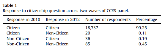
I wrote this post “fresh”–that is, without looking at what others had written about the study. Maggie Koerth at fivethirtyeight.com wrote an article in 2017 nicely summarizing the subsequent dust-up (including a sympathetic look at one of Richman’s co-authors, who was an undergraduate student when she worked on the paper). Richman et al.’s study has apparently been racked over the coals, with the CCES principal investigators chalking up Richman et al.’s findings to measurement error for citizenship status (although why the CCES PIs used the 2010/2012 CCES instead of the 2008/2010 CCES baffles me edit: I get it now; the 2012 CCES re-interviewed some of the 2010 respondents and they could doublecheck the citizenship status variable). I am also struck by John Ahlquist and Scott Gehlbach’s 2014 piece pointing out that the suprisingly high percentages of non-citizens reporting they are registered to vote may actually be referring to being registered to vote in their countries of origin.