The JupyterLab notebook of this post can be found here.
PyTorch has inherited simple, fast and efficient linear curve fitting capabilities from very well-known BLAS and LAPACK packages. These packages have extensive efficient linear algebra operations. Besides all the capabilities, there is a simple function, lstsq, which can solve linear least square or least norm problem. Least square solution is for over-determined system of linear equations and least norm is for under-determined system of linear equations. But this insignificant capability can be easily extend because of PyTorch. Two factors make this simple function very interesting; the ability to run on GPU because of PyTorch and also ability to add high degree of non-linearity with activation functions. Here we will use this two capacity to make very good quality curve fitters.
First step for any estimation is to produce data. Here we assume almost perfect condition on data; it means continues values without any missing data. The only impurity is additive Gaussian noise.
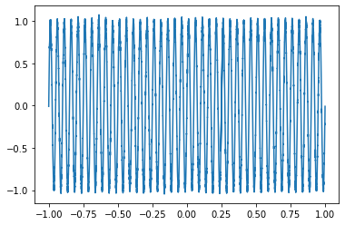
The curve which produces the data is a sine wave a fixed frequency.

The noise power can be changes by standard deviation of Gaussian random number generator.
All the models and tensors are sent to GPU to achieve high processing speed.
The curve fitting has been done in two ways:
- Fitting summation of non-linear functions with different degrees
Several activation functions have been tried. Degree or order of function has been defined differently for each function. For polynomials, order is the largest degree of the main variable. For geometrical functions like sine or cosine, the order is the same as frequency. And for tanh and sigmoid order is defined as the main variable multiplier. Most functions achieved the same results based on the situation. But the important observation has happened when the order of function increases around 50. The fitness break and the function started to go to infinity or a highly noisy behavior appeared. For preventing the noisy behavior, the order has been increased not by one, but two or five or ten. This removed the noisy behavior while keeping the mean square error almost fixed. But no solution could be found for tendency to infinity. When the data type changed from float32 to float64, it helps a little but not significantly. Therefore, when the shape of function is a little complex, increasing the order is one of the solutions which help the estimator to make a good fit, but if the function get too complex with many fluctuations, then since it wouldn’t be possible to increase the order, then the fitness is too unsuccessful. Then we think about local fitness which is discussed as follows.
- Fitting piece-wise summation of non-linear functions with low degrees
The idea of this method is simple; dividing the input variable range into several partition and fitting a simple estimator for each part separately. A function with high variation was successfully estimated with piece-wise estimation just by polynomials of order 3. Two parameters are important in this estimation; the number of partitions and order of function. The number of parameters which will be used for this method is the product of number of partitions and order of function. For example if the number of partitions would be 10 and order of polynomial function would be 3 (it means 4 coefficients), then the number of parameters for curve fitting would be 40. This method is fast and very efficient for a single variable. But if there would be 100 input dimensions and each one needs just 10 partitions with polynomial estimator of degree 3, then the number of required parameters would be:
3 * (10 ^ 100)
It is clear that this type of estimation would be just feasible for low dimensional problems.
Next step would be trying to use neural network for curve fitting where will be discussed in part 2.

Be First to Comment