Alternative Graphics Editor

As someone that is about to lose access to my Temple sponsored software one of the things I’m going to miss the most is Adobe Illustrator (AI). The Cartographic Design requirement for the PSM in GIS really made it clear how a few simple image adjustments using a program like Illustrator can make a map product exported from ArcGIS or QGIS look thousands of times better. Luckily while attending a recent Technical Workshop at Azavea one of the lightning talks was about improving product visualization. The speaker Jeff Frankl, User Experience Designer at Azavea demonstrated Figma.com, an online alternative to AI. Currently Figma is free to use as an individual, with the ability to have three active projects stored for 30 days. The user interface is very similar to AI, but if you’re new to both programs there are plenty of instructional videos, the major difference being that Figma projects can be shared online and worked on collaboratively.

There are also plenty of other free or low cost design products like Inkspace and GIMP there is a pretty thorough list available at this link.


Adding Citations to R Markdown

Versions of this blog entry are available as an HTML page, PDF and a text file containing the info from the Rmd file.  If you download the text file and save it with an .Rmd extension you will be able to create this document in R Markdown and edit it to fit your report requirements.

Abstract

Putting this section in between asterisks prints it out in italics. This blog goes shows you how to add citations to an Rmarkdown document.

Introduction

Adding citations is an important part of any complete document, this blog in addition to the previous entry about setting up an R markdown document should hopefully get you started.

Methods

  • Create a new R markdown document and save it with the file extension .Rmd to your working directory, which should be set somewhere convenient as you need to save other files to this location. Delete everything in that file but the info at the top in between the set of three dashes. Add a new line to that section ‘bibliography: bibliography.bib’.
  • You will need to save the references as a .bib file. Luckily for most items available from the Temple University Library system most journals and other items have an ‘Export citation’ look for something that says .bib or BibTex.
  • Save those files and open a new text file named bibliography.bib in your working directory, copy the data from the library file to your bibliography file. Example here
  • The format to create your own .bib file is written up very clearly here  if you can’t get the completed file from your source library.
  • In your text if you want to cite something just use the @ sign and brackets to wrap the name of the reference from the first line of the .bib data. This usually is just the author’s name underscore year.
  • For example writing [see @R_Core_Team_2017] produces (see R Core Team 2017)
  • Or just write @R_Core_Team_2017 so the text appears as part of the docume nt like this: as noted in R Core Team (2017)
  • References will show up at the bottom of your document after last text entry, so add a header and you’re done!

As an extra bonus R Studio has a spell-checking function- just hit F7

References

Osborne, Martin J. 2008. “Using Bibtex: A Short Guide.” https://www.economics.utoronto.ca/osborne/latex/BIBTEX.HTM.

R Core Team. 2017. R: A Language and Environment for Statistical Computing. Vienna, Austria: R
Foundation for Statistical Computing. https://www.R-project.org/.

Using R Markdown to Create Reports

Intro

Using R and Rstudio along with the R Markdown package allows you to produce documents in markdown that can be easily converted to MS Word, PDF, or saved as an HTML file that can be hosted as a website. The R Markdown file can contain just text like simple written report or a much more complex document with embedded R code to create charts, graphs, maps, or any other plot that can be produced using R. The text plots and formatting can all be created in a single document with a streamlined workflow. Instead of producing charts, tables, and graphs in MS Excel, and then placing those items in the text of a Word document, and then adding any other images (maps etc.) all that work can be completed in one place. If the report is required to be replicated with new data, it is simple to update the data rerun the code and produce a new version of the document.

Important links

The following preliminary steps should be taken before proceeding.
Download and install:
R https://cran.r-project.org/bin/windows/base/.
RSTUDIO https://www.rstudio.com/products/rstudio/download/#download.
To produce PDF documents you may also have to download and install pandoc, which is available here.

Package Installation

In the tools menu of RStudio click ‘Install packages’ and type Rmarkdown, make sure that the ‘install dependencies’ box is checked, that will also install some other important packages, including knitr.

For reference you can download the most recent Rmarkdown cheat sheet by navigating to the help menu and selecting the appropriate file under cheatsheets.

Once all of that is completed go to the file tab in RStudio and select new file -> R Markdown fill out the boxes and click okay on the window that pops up, that info can be updated later.

Save the new document that R Studio opens somewhere convenient and make sure the file ends in “.Rmd” (the case is very important here).

See the slightly darker bands? Those are called ‘code chunks’ within each chunk you can select various options via the gear symbol such as: to display the R code, to run and display the code, to not run or display code (this is used when you want to set up for an action completed later -like call a library), show or hide warnings in your final document etc.

The other sections are where you place your text. The text is formatted using the Pandoc format (summarized on the cheatsheet) which shows up after create the in your desired format. A # means Header size 1 and two spaces creates a paragraph break etc. You can play with the formatting of the sample page, add text and format a few lines to see how they come out.

Then select the small pull down at the top of the Source panel (where your new document appeared) that says Knitr and looks like a ball of yarn -there are options to Knit to HTML, PDF or Word,

From the Rmarkdown cheatsheet:
When you render, R Markdown
1. runs the R code, embeds results and text into .md file with knitr
2. then converts the .md file into the finished format with pandoc

Running R Code

Here is a flow chart of the R Markdown process which was included to show how to include plot made by the R code:

```{r, echo=TRUE}
DiagrammeR::DiagrammeR("graph LR;
 A(Rmd)-->B((knitr)); 
 B-->C{pandoc};
 C-->D>HTML];
 C-->E>PDF];
 C-->F>Word];")
 C-->F>Word];")
```

As far as I can tell WordPress does not allow for directly loading a .md file so versions of this blog entry are available as an HTML page, PDF and a text file containing the info from the Rmd file.

Flow charts in R using DiagrammeR

This is really short but I was really excited to share this info. When I was trying to find a way to create a flow chart in R I started with a few different packages that required a huge amount of prep work  before plotting a flow chart, and then I found the magical DiagrammeR  package.

It really should be more difficult:

library(DiagrammeR)
DiagrammeR("graph LR;
           A-->B;
           B-->C;
           B-->D")

Creates this:

Pretty cool, Right?

By assigning each letter you can update the flow direction, text and shape

DiagrammeR("graph TB;
    A(Rounded)-->B[Squared];
    B---C{Rhombus!};
    C-->D>flag shape];
    C-->E((Circle));")

Creates this:

Notice that after graph it says TB (top bottom) vs LR, Text can be added, type of brackets dictate the output shape and — vs –> makes a line instead of an arrow.

This package is really impressive and the documentation has some  very interesting images of very complicated graphs and flow charts, this image was made using the example provided in the package instructions.

R Shiny –Task: create an input select box that is dependent on a previous input choice.

The R shiny package is impressive, it gives you the power of R, plus any number of packages, and in combination with your data allows you to create a personalized web application without having to know any JavaScript. There are endless possibilities of display options, add-on widgets, and visualization possibilities. While working on another project I ran into a really simple problem that took way too long solve. I watched innumerable tutorials and read up on the documentation, but for some reason I could not get an input selector to display reactive data based on a previously selected input. The ability to narrow down an input is something that is encountered on websites daily when entering address fields- Enter Country; which drives the next pull-down menu to offer up a list of States, but it took a while to make it for me to get to work in a Shiny app.

In order to make someone’s life a bit easier here is an example that I cobbled together that offers up county names based on the State selected, here for brevity’s sake the example uses a table created in the R code that only includes Delaware and Rhode Island- no extra data is needed to be downloaded. As a bonus I added a plot output using the “maps” package to highlight the selected county. There is code to install the “map” package, the assumption is being made that if you’re this far the “shiny” package is already installed and you are doing all of this through RStudio.

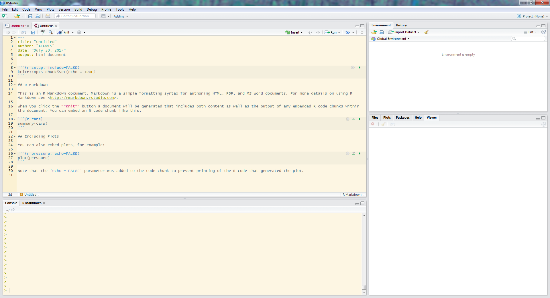
In RStudio paste the following code into a new file and name that file app.R so that RStudio recognizes it as a shiny app, as a best practice save it in a new folder that does not have any other files in it. Once saved as app.R the “Run” button at the top of the console should now say “Run App”. Click the “Run App” button and the app should load in a new window.

Breakdown of the file:
Section 1: runs once before the app is created and establishes the data in the app- could use this to upload a file, but in this example the datatable is created here.

Section 2: User interface(UI): this section sets up the appearance of the app, in this example the most important part was calling the input selectboxes using the “htmlOutput()” call that grabs information from the next section.

Section 3: Server: The “output$state_selector” uses the “renderUI()” call to utilize the “selectInput()” parameters set up the appearance and data in the state select input box of the UI. The second similar call “output$county_selector” uses the data from the state_selector call to filter the datatable and then this filtered data (now named “data_available”) is called by the second selectInput() command. Notice that each of the selectInput calls are wrapped in their own renderUI call. The last bit“output$plot1”, uses the info from the previous calls to display a map highlighting the selected county using the “renderPlot() call.

Section 4: make sure this is the last line of code in your file.

The following code is extensively commented, and should allow you to reuse as needed.

#install.packages( "maps", dependencies = TRUE) #run this to install R package maps
 ################################- warning this will update existing packages if already installed

#*save the following code in a file named app.R *
 library(shiny)
 library(maps)

##Section 1 ____________________________________________________
 #load your data or create a data table as follows:
 countyData = read.table(
 text = "State County
 Delaware Kent
 Delaware 'New Castle'
 Delaware Sussex
 'Rhode Island' Bristol
 'Rhode Island' Kent
 'Rhode Island' Newport
 'Rhode Island' Providence
 'Rhode Island' Washington",
 header = TRUE, stringsAsFactors = FALSE)

##Section 2 ____________________________________________________
 #set up the user interface
 ui = shinyUI(
 fluidPage( #allows layout to fill browser window
 titlePanel("Reactive select input boxes"),
 #adds a title to page and browser tab
 #-use "title = 'tab name'" to name browser tab
 sidebarPanel( #designates location of following items
 htmlOutput("state_selector"),#add selectinput boxs
 htmlOutput("county_selector")# from objects created in server
 ),

mainPanel(
 plotOutput("plot1") #put plot item in main area
           )
       ) )


 ##Section 3 ____________________________________________________
 #server controls what is displayed by the user interface
 server = shinyServer(function(input, output) {
 #creates logic behind ui outputs ** pay attention to letter case in names

output$state_selector = renderUI({ #creates State select box object called in ui
 selectInput(inputId = "state", #name of input
 label = "State:", #label displayed in ui
 choices = as.character(unique(countyData$State)),
 # calls unique values from the State column in the previously created table
 selected = "Delaware") #default choice (not required)
 })
 output$county_selector = renderUI({#creates County select box object called in ui

data_available = countyData[countyData$State == input$state, "County"]
 #creates a reactive list of available counties based on the State selection made

selectInput(inputId = "county", #name of input
 label = "County:", #label displayed in ui
 choices = unique(data_available), #calls list of available counties
 selected = unique(data_available)[1])
 })

output$plot1 = renderPlot({ #creates a the plot to go in the mainPanel
 map('county', region = input$state)
 #uses the map function based on the state selected
 map('county', region =paste(input$state,input$county, sep=','),
 add = T, fill = T, col = 'red')
 #adds plot of the selected county filled in red
 })
 })#close the shinyServer

##Section 4____________________________________________________
 shinyApp(ui = ui, server = server) #need this if combining ui and server into one file.


See the wonder live at shinyapps.io

Find the best matched polygons for use in a time series using pgAdmin

Goal:
Find the best matched polygons in a time series using a PostGIS Spatial Database
Background:
For previous project a comparison of housing data from the 1930s to current and historic US Census data was required. The geographic portion of the census data, was obtained from the National Historical Geographic Information System (NHGIS) which produces downloadable shapefiles with a GISJOIN field allowing for convenient linking of the shapefile to tables of census data also available through NHGIS. The 1930s housing data was in the form of an image of a 1937 Home Owners’ Loan Corporation (HOLC) map of Philadelphia available here. Very broadly the HOLC graded neighborhoods based on race/class and these grades where then used to determine the likelihood of housing loan assistance. There is debate if the HOLC process normalized race-based home lending practices and then the lead to further housing issues such as redlining. more info.

Process:
The HOLC map data was pulled into a GIS and a shapefile was created of the neighborhood grading (this process is often listed as ‘Heads-up Digitizing’ in job postings) here is a handy tutorial for ArcMap and another using QGIS. Shapefile and HOLC jpeg available on github.

The HOLC neighborhood grading schema does not coincide with any current (or historic) census arrangement so the spatial querying capabilities of pgAdmin and the PostgreSQL database engine was used to match the newly created HOLC digital data with the NHGIS Decennial Census geographic data.
Create a PostGIS Spatial Database and use pgShapeLoader to load the shapefiles (HOLC and NHGIS spatial data)

After much trial and error the following code worked the best:

create table overlap2010census as
with limited as(
select distinct us2010.*
from us2010, holc1937
WHERE ST_DWithin(us2010.geom, holc1937.geom, 0.25)
order by us2010.gid
)
/* the section above limits the query of the 2010 census polygons (Entire US) to those near the HOLC polygons –input can vary based on projection of files*/

SELECT DISTINCT ON (limited.gid)
limited.gid as us2010a_gid,
holc1937.gid as holc_gid, holc1937.name, holc1937.grade,
st_area((st_transform(limited.geom,4326)::geography)) as area_check,
ST_Area(ST_Intersection((st_transform(limited.geom,4326)::geography),
(st_transform(holc1937.geom,4326)::geography))) as intersect_area_2010_meters,
(ST_Area(ST_Intersection((st_transform(limited.geom,4326)::geography),
(st_transform(holc1937.geom,4326)::geography)))/
st_area((st_transform(limited.geom,4326)::geography)))*100 as percent_overlap,

/*calculates the area of the returned census and HOLC polygons and the percent of overlap */

limited.*
FROM limited, holc1937
where limited.geom && ST_Expand(holc1937.geom,1) and ST_Area(ST_Intersection(limited.geom, holc1937.geom)) >0

/* joins the files where the geom overlap*/

ORDER BY limited.gid, ST_Area(ST_Intersection((st_transform(limited.geom,4326)::geography),
(st_transform(holc1937.geom,4326)::geography))) DESC;

/* sorts by the largest amount of overlap, and in conjunction with the DISTINCT ON call
only returns the first instance of the census polygon that overlaps the target polygon */

While this method requires the user to update and repeat this code for each comparison the tables created can then be exported out to your GIS or QGIS can connect directly to your database if you prefer that option. As the query also created a unique identifier for each year and polygon of the Census data, a crosswalk/key table was created using this data which allowed for the Census data (race,income housing status etc.) for multiple years to be attached via the NHGIS GISJOIN field previously mentioned. Based off of the multiyear Census data attached via the crosswalk table comparisons of the HOLC geographic areas could then be made regardless of shifting Census borders.